7 Formal concept analysis

7.1 Formal Concept Analysis in `R`

FCA is a mathematical tool based on lattice theory and logic. It is the forgotten sister in data science.

However, FCA allows to discover hidden knowledge in a dataset in a similar (or even more powerful) way than some very famous Machine Learning techniques such as, for example, association rules.

Why develop an R package for FCA?

Helping to disseminate FCA as a new knowledge discovery tool
Help to integrate methods from different areas that do not really have empty intersection
Help the more theoretical FCA community to calculate concepts, implications, minimal generators, etc.
Applying FCA to real problems: development of recommender systems in tourism and medicine

For us it is useful to:

disseminate our theoretical works to a wider audience not only in the FCA community
close the cycle: theory-practice-theory.

7.2 Any rule management packages?

arules
frbs
RKEEL

We highlight arules well known in the data science community for extracting and managing patterns and association rules.

7.3 The `fcaR` package

The package is in a stable phase in a repository on Github and on CRAN.

Unit tests
Bullets with demos
Status:
- lifecycle: stable
- CRAN: 1.1.1
- build: passing
- downloads: ~13K
Installation:

# Latest version
remotes::install_github("Malaga-FCA-group/fcaR", build_vignettes = TRUE)

# Stable version
install.packages("fcaR")

The package is also available from CRAN.

7.4 Extensibility

Object-oriented programming: extensible classes.
Use of registry to extend functionality:
- Redundancy elimination methods.
- Methods for constructing the concept lattice.
- Techniques for finding the implication base.

7.5 `fcaR`

The first important issue regarding transaction datasets used in association rules: in association rules the datasets are either binary or with categorical or discrete information that can be passed to binary.

FCA is able to work with binary or fuzzy information stored in the datasets and extract implications (association rules with confidence one) and also a concept lattice.

7.5.1 Formal Context

We will use the following binary dataset called planets which appears in:

Wille R (1982). “Restructuring Lattice Theory: An Approach Based on Hierarchies of Concepts.” In Ordered Sets, pp. 445–470. Springer.

knitr::kable(planets, format = "html", booktabs = TRUE)

	small	medium	large	near	far	moon	no_moon
Mercury	1	0	0	1	0	0	1
Venus	1	0	0	1	0	0	1
Earth	1	0	0	1	0	1	0
Mars	1	0	0	1	0	1	0
Jupiter	0	0	1	0	1	1	0
Saturn	0	0	1	0	1	1	0
Uranus	0	1	0	0	1	1	0
Neptune	0	1	0	0	1	1	0
Pluto	1	0	0	0	1	1	0

We create a formal context from the above dataset using the fcaR package:

library(fcaR)
fc_planets <- FormalContext$new(planets)
fc_planets$print()
## FormalContext with 9 objects and 7 attributes.
##          small  medium  large  near  far  moon  no_moon  
##  Mercury   X                     X                 X     
##    Venus   X                     X                 X     
##    Earth   X                     X          X            
##     Mars   X                     X          X            
##  Jupiter                  X           X     X            
##   Saturn                  X           X     X            
##   Uranus           X                  X     X            
##  Neptune           X                  X     X            
##    Pluto   X                          X     X

In the formal context fc_planets we have some properties and methods that can be used to extract hidden knowledge in the dataset.

fc_planets$dim()
## [1] 9 7
fc_planets$attributes
## [1] "small"   "medium"  "large"   "near"    "far"     "moon"    "no_moon"
fc_planets$objects
## [1] "Mercury" "Venus"   "Earth"   "Mars"    "Jupiter" "Saturn"  "Uranus" 
## [8] "Neptune" "Pluto"
fc_planets$plot()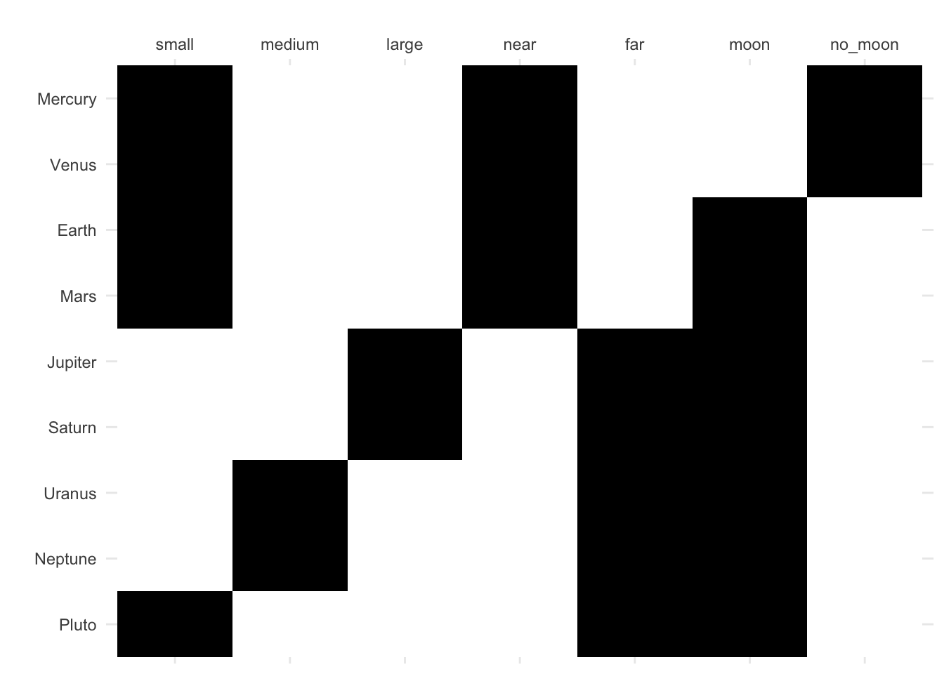

For Latex users:

fc_planets$to_latex(table = FALSE)
## \begin{tabular}{r|ccccccc}
##   & $small$ & $medium$ & $large$ & $near$ & $far$ & $moon$ & $no\_moon$\\ 
##  \hline 
##  $Mercury$ & $\times$ &  &  & $\times$ &  &  & $\times$ \\
## $Venus$ & $\times$ &  &  & $\times$ &  &  & $\times$ \\
## $Earth$ & $\times$ &  &  & $\times$ &  & $\times$ &  \\
## $Mars$ & $\times$ &  &  & $\times$ &  & $\times$ &  \\
## $Jupiter$ &  &  & $\times$ &  & $\times$ & $\times$ &  \\
## $Saturn$ &  &  & $\times$ &  & $\times$ & $\times$ &  \\
## $Uranus$ &  & $\times$ &  &  & $\times$ & $\times$ &  \\
## $Neptune$ &  & $\times$ &  &  & $\times$ & $\times$ &  \\
## $Pluto$ & $\times$ &  &  &  & $\times$ & $\times$ &  
##  \end{tabular}

7.5.2 Concepts

We can calculate concepts using Ganter and Wille’s NextClosure algorithm, implemented in the find_concepts() method, which is developed in C behind R.

fc_planets$find_concepts()
fc_planets$concepts$size()
## [1] 12
head(fc_planets$concepts)
## A set of 6 concepts:
## 1: ({Mercury, Venus, Earth, Mars, Jupiter, Saturn, Uranus, Neptune, Pluto}, {})
## 2: ({Earth, Mars, Jupiter, Saturn, Uranus, Neptune, Pluto}, {moon})
## 3: ({Jupiter, Saturn, Uranus, Neptune, Pluto}, {far, moon})
## 4: ({Jupiter, Saturn}, {large, far, moon})
## 5: ({Uranus, Neptune}, {medium, far, moon})
## 6: ({Mercury, Venus, Earth, Mars, Pluto}, {small})

FCA showed that there is an ordering relationship in the concepts.
A concept lattice (concept taxonomy) has actually been calculated.

7.5.2.1 Plot of the concept lattice

fc_planets$concepts$plot(object_names = FALSE)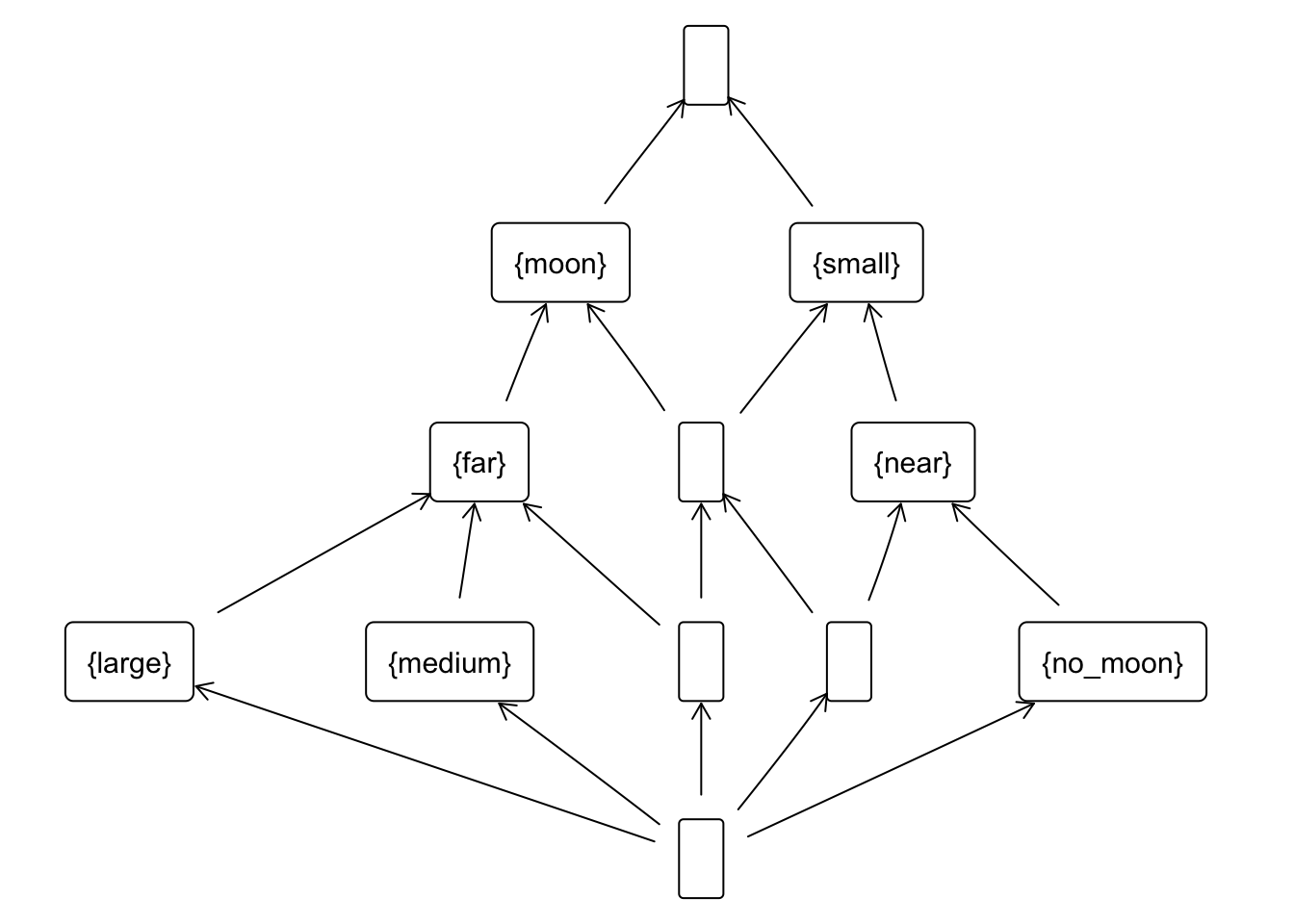

fc_planets$concepts$sub(2)
## ({Earth, Mars, Jupiter, Saturn, Uranus, Neptune, Pluto}, {moon})

There is a set of planets with common characteristics - we have discovered hidden knowledge: does this concept already have a name?

A concept $(A, B)$, contains a set of objects $A$ (the extent) and a set of attributes $B$ (the intent) such that:

the extent $A$ consists of all objects that share the attributes in $B$.
the intent $B$ consists of all the attributes shared by the objects in $A$.

7.5.2.2 Closures

The basic operation in FCA is the calculation of closures from a set of attributes or from a set of objects. Two mathematical functions (two derivation operators) are used, which we have called in our library extent() (from objects), intent() (from attributes).

The extent() of a set of objects is the set of their common attributes:

# Define a set of objects
S <- Set$new(attributes = fc_planets$objects)
S$assign(Earth = 1, Mars = 1)
S
## {Earth, Mars}

# Compute the intent of S
fc_planets$intent(S)
## {small, near, moon}

With this we can see what common properties Earth and Mars have in common.

Analogously, the intent() of an attribute set is the set of objects that possesses all the attributes in the set:

# Define a set of objects
S <- Set$new(attributes = fc_planets$attributes)
S$assign(moon = 1, large = 1)
S
## {large, moon}

# Compute the extent of S
fc_planets$extent(S)
## {Jupiter, Saturn}

Planets that have the characteristics indicated.

7.5.2.3 Operations with the lattice

All basic functions developed in the FCA theory by Ganter and Wille have been implemented:

fc_planets$concepts$support()
##  [1] 1.0000000 0.7777778 0.5555556 0.2222222 0.2222222 0.5555556 0.3333333
##  [8] 0.1111111 0.4444444 0.2222222 0.2222222 0.0000000

# Get the index of those concepts with support 
# greater than the threshold
idx <- which(fc_planets$concepts$support() > 0.2)
# Build the sublattice
sublattice <- fc_planets$concepts$sublattice(idx)
sublattice
## A set of 12 concepts:
## 1: ({Mercury, Venus, Earth, Mars, Jupiter, Saturn, Uranus, Neptune, Pluto}, {})
## 2: ({Earth, Mars, Jupiter, Saturn, Uranus, Neptune, Pluto}, {moon})
## 3: ({Jupiter, Saturn, Uranus, Neptune, Pluto}, {far, moon})
## 4: ({Jupiter, Saturn}, {large, far, moon})
## 5: ({Uranus, Neptune}, {medium, far, moon})
## 6: ({Mercury, Venus, Earth, Mars, Pluto}, {small})
## 7: ({Earth, Mars, Pluto}, {small, moon})
## 8: ({Pluto}, {small, far, moon})
## 9: ({Mercury, Venus, Earth, Mars}, {small, near})
## 10: ({Mercury, Venus}, {small, near, no_moon})
## 11: ({Earth, Mars}, {small, near, moon})
## 12: ({}, {small, medium, large, near, far, moon, no_moon})
sublattice$plot()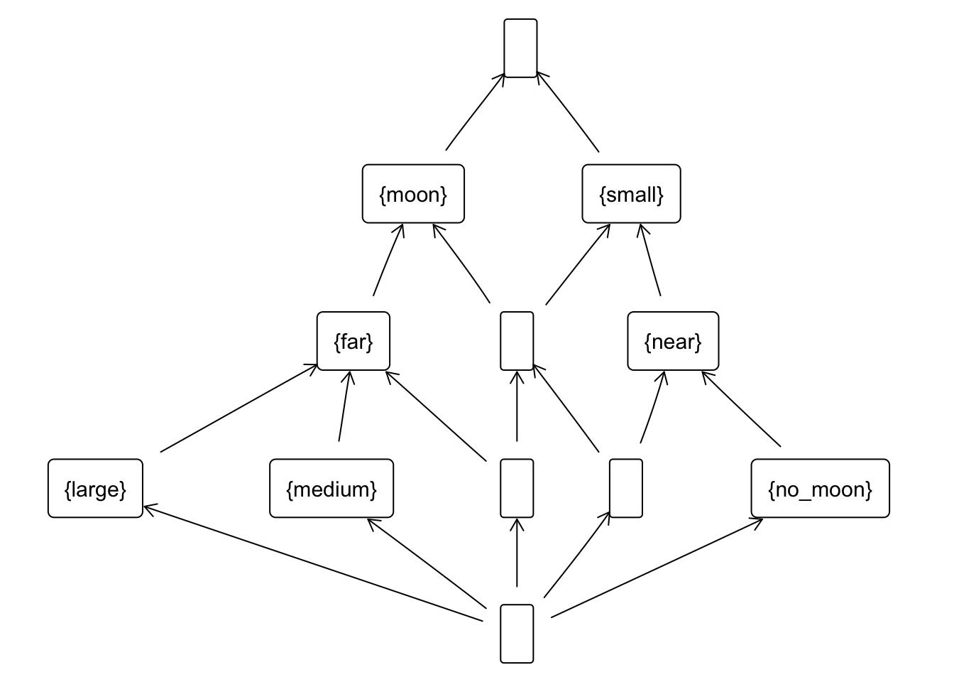

# The fifth concept
C <- fc_planets$concepts$sub(5)
C
## ({Uranus, Neptune}, {medium, far, moon})
# Its subconcepts:
fc_planets$concepts$subconcepts(C)
## A set of 2 concepts:
## 1: ({Uranus, Neptune}, {medium, far, moon})
## 2: ({}, {small, medium, large, near, far, moon, no_moon})
# And its superconcepts:
fc_planets$concepts$superconcepts(C)
## A set of 4 concepts:
## 1: ({Mercury, Venus, Earth, Mars, Jupiter, Saturn, Uranus, Neptune, Pluto}, {})
## 2: ({Earth, Mars, Jupiter, Saturn, Uranus, Neptune, Pluto}, {moon})
## 3: ({Jupiter, Saturn, Uranus, Neptune, Pluto}, {far, moon})
## 4: ({Uranus, Neptune}, {medium, far, moon})
# A list of concepts
C <- fc_planets$concepts[5:7]
C
## A set of 3 concepts:
## 1: ({Uranus, Neptune}, {medium, far, moon})
## 2: ({Mercury, Venus, Earth, Mars, Pluto}, {small})
## 3: ({Earth, Mars, Pluto}, {small, moon})
# Supremum of the concepts in C
fc_planets$concepts$supremum(C)
## ({Mercury, Venus, Earth, Mars, Jupiter, Saturn, Uranus, Neptune, Pluto}, {})
# Infimum of the concepts in C
fc_planets$concepts$infimum(C)
## ({}, {small, medium, large, near, far, moon, no_moon})
fc_planets$concepts$join_irreducibles()
## A set of 5 concepts:
## 1: ({Jupiter, Saturn}, {large, far, moon})
## 2: ({Uranus, Neptune}, {medium, far, moon})
## 3: ({Pluto}, {small, far, moon})
## 4: ({Mercury, Venus}, {small, near, no_moon})
## 5: ({Earth, Mars}, {small, near, moon})
fc_planets$concepts$meet_irreducibles()
## A set of 7 concepts:
## 1: ({Earth, Mars, Jupiter, Saturn, Uranus, Neptune, Pluto}, {moon})
## 2: ({Jupiter, Saturn, Uranus, Neptune, Pluto}, {far, moon})
## 3: ({Jupiter, Saturn}, {large, far, moon})
## 4: ({Uranus, Neptune}, {medium, far, moon})
## 5: ({Mercury, Venus, Earth, Mars, Pluto}, {small})
## 6: ({Mercury, Venus, Earth, Mars}, {small, near})
## 7: ({Mercury, Venus}, {small, near, no_moon})

7.5.3 Implications. Duquenne-Guigues basis

The NextClosure algorithm is used to compute at the same cost not only concepts but also implications.

The find_implications() method is applied to a *formal context object (of class FormalContext).

fc_planets$find_implications()

The result (a set of association rules with confidence 1) is stored in fc_planets$implications.

fc_planets$implications$cardinality()
## [1] 10
fc_planets$implications
## Implication set with 10 implications.
## Rule 1: {no_moon} -> {small, near}
## Rule 2: {far} -> {moon}
## Rule 3: {near} -> {small}
## Rule 4: {large} -> {far, moon}
## Rule 5: {medium} -> {far, moon}
## Rule 6: {medium, large, far, moon} -> {small, near, no_moon}
## Rule 7: {small, near, moon, no_moon} -> {medium, large, far}
## Rule 8: {small, near, far, moon} -> {medium, large, no_moon}
## Rule 9: {small, large, far, moon} -> {medium, near, no_moon}
## Rule 10: {small, medium, far, moon} -> {large, near, no_moon}
fc_planets$implications[2:4]
## Implication set with 3 implications.
## Rule 1: {far} -> {moon}
## Rule 2: {near} -> {small}
## Rule 3: {large} -> {far, moon}

7.5.3.1 Simplification Logic in `R`

We propose Simplification Logic as a tool for developing automatic reasoning methods.

For the case of binary datasets, we have proposed (Ángel Mora, Pablo Cordero, Manuel Enciso, et. al.) the Logic of Simplifications, in 2012.

Axiom: infer $A\cup B\Rightarrow A$
Multiplication: from $A\Rightarrow B$ infer $c^*{\otimes}A\Rightarrow c^*{\otimes}B$
Simplification: from $A \Rightarrow B$ and $C \Rightarrow D$ infer $(C\smallsetminus B) \Rightarrow (D\smallsetminus B)$ if $A\subseteq C$
Rsimplification: from $A \Rightarrow B$ and $C \Rightarrow D$ infer $C \Rightarrow (D\smallsetminus B)$ if $A\subseteq (C \cup D)$

The Simplifications Logic is the engine of automatic methods for:

Elimination of redundancy,
Calculation of attribute closures,
Minimal key calculation,
Obtaining recommendations, etc.

In fcaR the following equivalence rules have been implemented, based on the axioms of logic:

Reduction: from $A\Rightarrow B$, infer $A\Rightarrow B\smallsetminus A$
Generalization: from $A\Rightarrow B$ and $C\Rightarrow D$, if $A\subseteq C$ and $D\subseteq B$, remove $C\Rightarrow D$.
Composition: if $A\Rightarrow B$ and $A\Rightarrow C$, replace both implications by $A\Rightarrow B\cup C$.
Simplification: if $A\Rightarrow B$ and $C\Rightarrow D$, with $A\subset C$ and $A\cap B = \emptyset$, replace $C\Rightarrow D$ by $C\smallsetminus B\Rightarrow D\smallsetminus B$.

fc_planets$plot()
# Average number of attributes on left and right hand side
colSums(fc_planets$implications$size())
# We apply the logic of simplification
fc_planets$implications$apply_rules(c("reduction",
                                      "composition",
                                      "generalization",
                                      "simplification",
                                      "rsimplification"))
# Average number of attributes in left and right hand side, after simplification
colSums(fc_planets$implications$size())

7.5.4 Support for the `arules` package

Import/Export transactions from arules.
Import rules from arules.
Manipulate the rules with our algorithms (use Simplification Logic, closures, etc.).
Subsequently export to arules.

library(arules)
## Loading required package: Matrix
## Warning: package 'Matrix' was built under R version 4.3.1
## 
## Attaching package: 'Matrix'
## The following object is masked from 'package:fcaR':
## 
##     %&%
## 
## Attaching package: 'arules'
## The following objects are masked from 'package:base':
## 
##     abbreviate, write
data("Mushroom")
rules_apriori <- apriori(Mushroom, parameter = list(support = 0.3, confidence = 1))
## Apriori
## 
## Parameter specification:
##  confidence minval smax arem  aval originalSupport maxtime support minlen
##           1    0.1    1 none FALSE            TRUE       5     0.3      1
##  maxlen target  ext
##      10  rules TRUE
## 
## Algorithmic control:
##  filter tree heap memopt load sort verbose
##     0.1 TRUE TRUE  FALSE TRUE    2    TRUE
## 
## Absolute minimum support count: 2437 
## 
## set item appearances ...[0 item(s)] done [0.00s].
## set transactions ...[114 item(s), 8124 transaction(s)] done [0.00s].
## sorting and recoding items ... [26 item(s)] done [0.00s].
## creating transaction tree ... done [0.00s].
## checking subsets of size 1 2 3 4 5 6 7 8 9 done [0.00s].
## writing ... [4059 rule(s)] done [0.00s].
## creating S4 object  ... done [0.00s].
inspect(head(rules_apriori))
##     lhs                      rhs                 support   confidence coverage 
## [1] {}                    => {VeilType=partial}  1.0000000 1          1.0000000
## [2] {GillSize=narrow}     => {RingNumber=one}    0.3092073 1          0.3092073
## [3] {GillSize=narrow}     => {GillAttached=free} 0.3092073 1          0.3092073
## [4] {GillSize=narrow}     => {VeilType=partial}  0.3092073 1          0.3092073
## [5] {CapSurf=smooth}      => {VeilType=partial}  0.3146233 1          0.3146233
## [6] {RingType=evanescent} => {GillAttached=free} 0.3417036 1          0.3417036
##     lift     count
## [1] 1.000000 8124 
## [2] 1.084936 2512 
## [3] 1.026535 2512 
## [4] 1.000000 2512 
## [5] 1.000000 2556 
## [6] 1.026535 2776

7.5.4.1 `arules` to `fcaR`

fc_Mushroom <- FormalContext$new(Mushroom)
fc_Mushroom$implications$add(rules_apriori)
fc_Mushroom$implications[2:5]
## Implication set with 4 implications.
## Rule 1: {GillSize=narrow} -> {RingNumber=one}
## Rule 2: {GillSize=narrow} -> {GillAttached=free}
## Rule 3: {GillSize=narrow} -> {VeilType=partial}
## Rule 4: {CapSurf=smooth} -> {VeilType=partial}
fc_Mushroom$implications$cardinality()
## [1] 4059
fc_Mushroom$implications$apply_rules(c(
  "reduction",
  "composition",
  "generalization",
  "simplification",
  "rsimplification"
))
## Processing batch
## --> Reduction: from 4059 to 4059 in 0.001 secs.
## --> Composition: from 4059 to 2168 in 0.241 secs.
## --> Generalization: from 2168 to 71 in 0.087 secs.
## --> Simplification: from 71 to 55 in 0.048 secs.
## --> Right Simplification: from 55 to 55 in 0.049 secs.
## Batch took 0.427 secs.
fc_Mushroom$implications$cardinality()
## [1] 55

7.5.4.2 `fcaR` to `arules`

arules_rules <- fc_Mushroom$implications$to_arules()
arules_rules
## set of 55 rules
class(arules_rules)
## [1] "rules"
## attr(,"package")
## [1] "arules"

7.5.5 Recommender system for medical diagnostics

7.5.5.1 Dataset `cobre32`

A diagnostic system from a formal context containing fuzzy medical data.

The dataset cobre32 has:

105 objects (patients) in rows.
30 attributes related to signs or symptoms, and 2 attributes related to diagnosis: dx_ss (strict schizophrenia) and dx_other (bipolar or schizoaffective disorder).

For each symptom-related attribute, there are several possible grades, from absent to extreme, through minimal, mild, moderate, moderate severe and severe, which are mapped into the interval $[0, 1]$.

data("cobre32")
colnames(cobre32)
##  [1] "COSAS_1"   "COSAS_2"   "COSAS_3"   "COSAS_4"   "COSAS_5"   "COSAS_6"  
##  [7] "COSAS_7"   "FICAL_1"   "FICAL_2"   "FICAL_3"   "FICAL_4"   "FICAL_5"  
## [13] "FICAL_6"   "FICAL_7"   "FICAL_8"   "FICAL_9"   "SCIDII_10" "SCIDII_11"
## [19] "SCIDII_12" "SCIDII_13" "SCIDII_14" "SCIDII_15" "SCIDII_16" "SCIDII_17"
## [25] "SCIDII_18" "SCIDII_19" "SCIDII_20" "SCIDII_21" "SCIDII_22" "SCIDII_23"
## [31] "dx_ss"     "dx_other"

# We create the formal context
fc <- FormalContext$new(cobre32)

# We extract both the concept lattice and the set of implications.
fc$find_implications()
fc$concepts$size()
## [1] 14706
fc$implications$cardinality()
## [1] 985

# We can apply equivalences to get a simpler set of implications.
fc$implications$apply_rules(rules = c("composition", "simplification"))
## Processing batch
## --> Composition: from 985 to 985 in 0.004 secs.
## --> Simplification: from 985 to 985 in 0.123 secs.
## Batch took 0.127 secs.
fc$implications$cardinality()
## [1] 985

7.5.5.2 Recommendations

From the extracted set of rules, we can define a function that encapsulates the behaviour of the recommender system:

# Here S is the set of known attributes for a new individual.
# Taking the implications, the consequent containing one of the possible diagnoses is calculated.
diagnose <- function(S) {
              fc$implications$recommend(S = S,
                                        attribute_filter = c("dx_ss","dx_other"))
  
}

Let’s see how it works with some examples.

Let us consider a first patient:

# We create a vector (set) for the patient's attributes
Patient1 <- Set$new(attributes = fc$attributes)

# We add those that are known
# (absent = 0, extreme = 1,...)
Patient1$assign(COSAS_1 = 0.5,
                COSAS_2 = 1,
                COSAS_3 = 0.5,
                COSAS_4 = 0.166667,
                COSAS_5 = 0.5,
                COSAS_6 = 1)
  
# Finally, we can run the recommender system
diagnose(Patient1) 
##    dx_ss dx_other 
##        1        0

The result tells us that this patient should be diagnosed as strict schizophrenia.

A second patient:

# Empty set
Patient2 <- Set$new(attributes = fc$attributes)

# We add the symptoms or signs:
Patient2$assign(FICAL_2 = 1)

# And we diagnose using the implication-based system.
diagnose(Patient2) 
##    dx_ss dx_other 
##        0        0

In this case, the sign that has been evaluated in this patient does not indicate (according to the set of implications that model the knowledge of the problem) any diagnosis. The problem remains open, and we will see how to solve it later.

Finally, a third patient:

Patient3 <- Set$new(attributes = fc$attributes)

Patient3$assign(COSAS_4 = 0.6666667,
                FICAL_3 = 0.5,
                FICAL_5 = 0.5,
                FICAL_8 = 0.5)
  

diagnose(Patient3) 
##    dx_ss dx_other 
##        0        1

In this case, the patient could be diagnosed with a disorder other than strict schizophrenia.

7.5.5.3 Closure with Simplification Logic - more knowledge

When we calculate the closure of a set of attributes using Simplification Logic, we also reduce the set of implications that contain important knowledge (this is the core of other automated methods).

This therefore provides us with additional knowledge that helps us to solve the problem that appeared earlier in Patient2.

# Here we get not only the closure, but a simplified subset of the implications that are relevant
cl <- fc$implications$closure(Patient2, 
                              reduce = TRUE)

# We write the first rules
new_rules <- cl$implications$filter(rhs = c("dx_ss", "dx_other"), 
                                    drop = TRUE)

new_rules[c(2, 5, 12:16)]
## Implication set with 7 implications.
## Rule 1: {SCIDII_19 [0.33]} -> {dx_ss, dx_other}
## Rule 2: {SCIDII_13 [0.33]} -> {dx_ss, dx_other}
## Rule 3: {SCIDII_14} -> {dx_ss}
## Rule 4: {SCIDII_14, SCIDII_18} -> {dx_other}
## Rule 5: {FICAL_1 [0.33], FICAL_4 [0.33], SCIDII_10 [0.5], SCIDII_18 [0.5],
##   dx_ss} -> {dx_other}
## Rule 6: {COSAS_7 [0.33]} -> {dx_ss, dx_other}
## Rule 7: {COSAS_6 [0.5], SCIDII_20 [0.5], dx_ss} -> {dx_other}

Some of these inferred rules can help physicians make the diagnosis.

7.1 Formal Concept Analysis in R