6 Association rules

Unsupervised learning: a technique that allows learning from observations to extract patterns, trends and make predictions - without prefixing a target.
Among the most relevant problems - prediction of customer behaviour, shopping trends: online shops, online services offering music, movies, etc.
Current reality is that there is a lot of competition, many similar services, online marketplaces, etc.
Objective: Attracting customers is the key.
Means: data collected from consumers, service users, consumer characteristics extracted from the collected data, previous purchase or usage patterns, etc.
Tools: Data Science methods - search for frequent patterns, rules, etc..

Applications:

Help personalise services and the shopping experience, guessing and suggesting shopping trends from likes, dislikes.
Analyse combinations of products that people tend to buy together.
Analyse reviews and prices that competitors offer for the same products.
Discovering customer habits by finding relationships between different items that consumers place in their shopping basket in the items that consumers place in their shopping basket in large supermarkets.
Analysis of purchases in large on-line shops - Amazon (thousands of products with millions of consumers), Google, etc., with the aim of (thousands of products with millions of consumers), Google, etc., with the objective of to offer recommendations.
Detect relationships to provide suggestions between songs, series, films, etc. that a consumer is interested in, films, etc. that a user listens to/watches in an online music internet application, or online music, or video internet application - Spotify, Netflix (25 million users), HBO, etc.
Control the peak hours of services.
Marketing, catalogue design.
Loan analysis, fraud detection, etc.

The problems in this area arise from the so-called Market Basket Analysis which deals with how to make product-based recommendations. Solutions for this problem can be used in other similar problems: recommendations of people’s interests, etc.

The most important techniques are:

Evaluation of the contingency matrix of the products.
Generation of frequent itemsets.
Extraction of association rules.

6.1 Detecting and predicting trends

Trend: specific pattern or buying and selling behaviour that appears over a period of time in a shop.
How to detect: Store all transactions that take place in the shop.
- items purchased
- stocks
- combinations of items bought together
- transaction of each sale made
How to process the data:
- pre-process
- normalise
- aggregate
Apply algorithms: spot patterns and trends.
Recommend: use patterns and trends to suggest new purchases.

The main method to achieve all this is based on the so-called Market Basket Analysis problem. These methods are based on probability-based statistics and probabilistic notions such as: * support * confidence * lift, etc.

Objective: Which items (products) have been purchased most frequently?

6.2 Fundamentals

6.2.1 Pattern search

Objective: to find relationships between data: market baskets, graphs, streams, etc.

They are the core element in many techniques in many different areas from database, AI, data mining, machine learning, etc. database, AI, data mining, machine learning, etc.
Frequent pattern search methods emerge in the area of data mining.
The first algorithm to be highlighted was the so-called Apriori algorithm.

They arise with the study of the so-called Market Basket Analysis.

Find coincidences between products purchased at the same time.

Predict when the purchase of one product may increase the purchase of others.

Stories - Beer and Diapers

6.3 Structure of transactions

Data: Typically a binary sparse D matrix of very large size.
Item: Each dataset column. A piece of data in the dataset that can be an attribute, a product, a disease, a word, a document, a biomarker, etc.
Transaction: Each row of the dataset typically representing a buyer, a pacient, a tweet, words in a document, genes, etc.
Itemset: A collection of zero or more items.

\(D_{i,j}\) represents item \(j\) in transaction \(i\).

Objective: Given a new bit vector representing what the consumer has bought, the aim is to predict what other products the consumer might be interested in buying.

Recommender systems.
Modelling dependencies in complex sw complex systems: if the consumer is interested in the product, it is possible to predict what other products he/she might be interested in buying.

Example

FormalContext with 5 objects and 6 attributes.
    frankfurter  sausage  liver loaf  ham  meat  finished products  
 t1                            X             X           X          
 t2                 X                                               
 t3                 X                  X                 X          
 t4                                          X                      
 t5                                                      X

6.3.1 First problem: Frequent Itemsets

The problem is to determine which sets of items occur jointly in the dataset. For instance, buying {beer, diapers, milk}.

This is a hard problem since we have to search a very complex space of possible itemsets.

But, we will have a good structure: a lattice. On the top we have the items (products), and in the second level combination of two-items, etc.

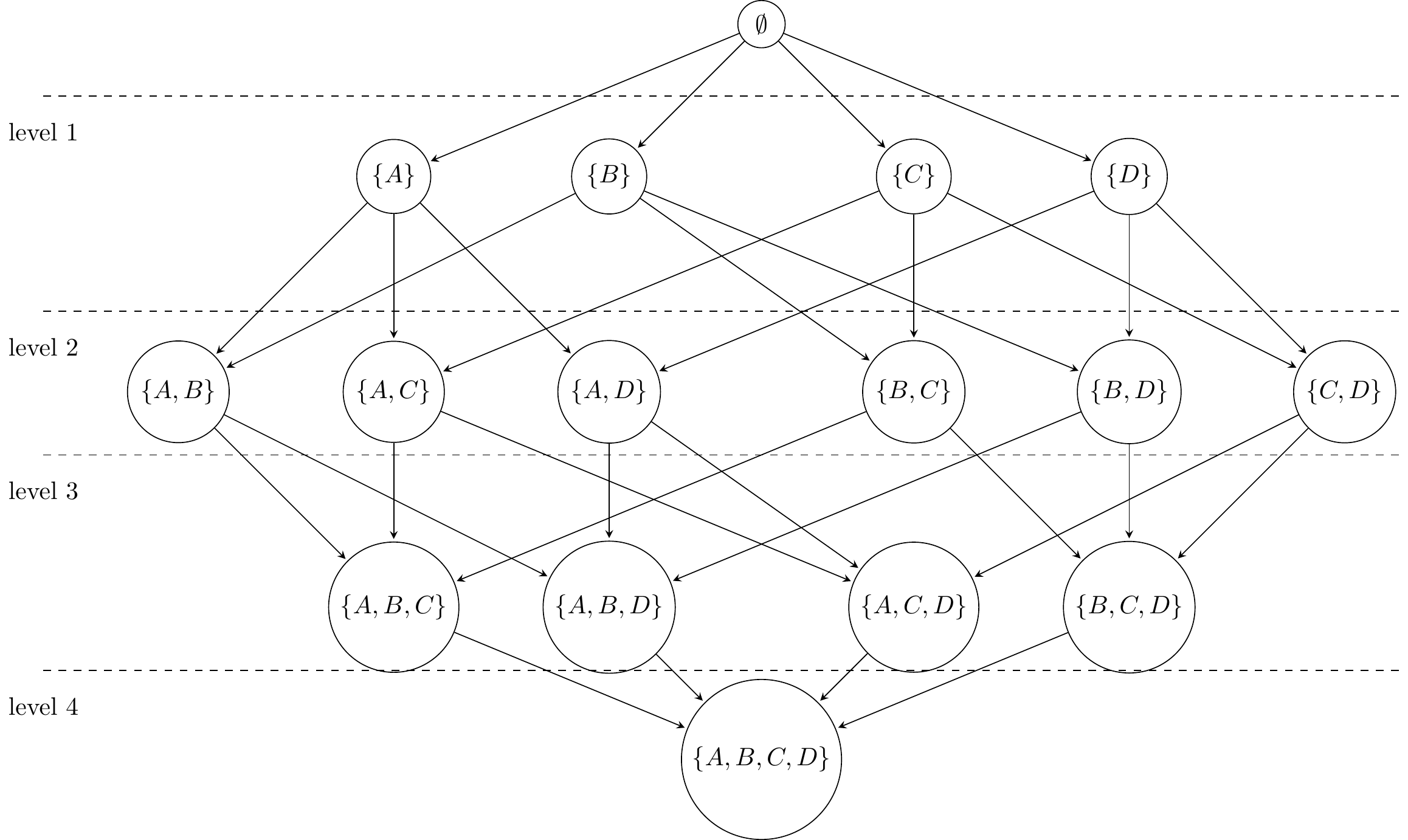
The idea is to simplify the search space by imposing a minimum support: A measure of the percentage of the pattern found in relation to the size of the dataset.

Notion: Frequent itemset - Set a threshold for the support that must be satisfied by the itemset found.

Support of an itemset is the proportion of transactions that have that itemset in the whole table:

\[Sup(X) = \frac{|X|}{|D|}\]

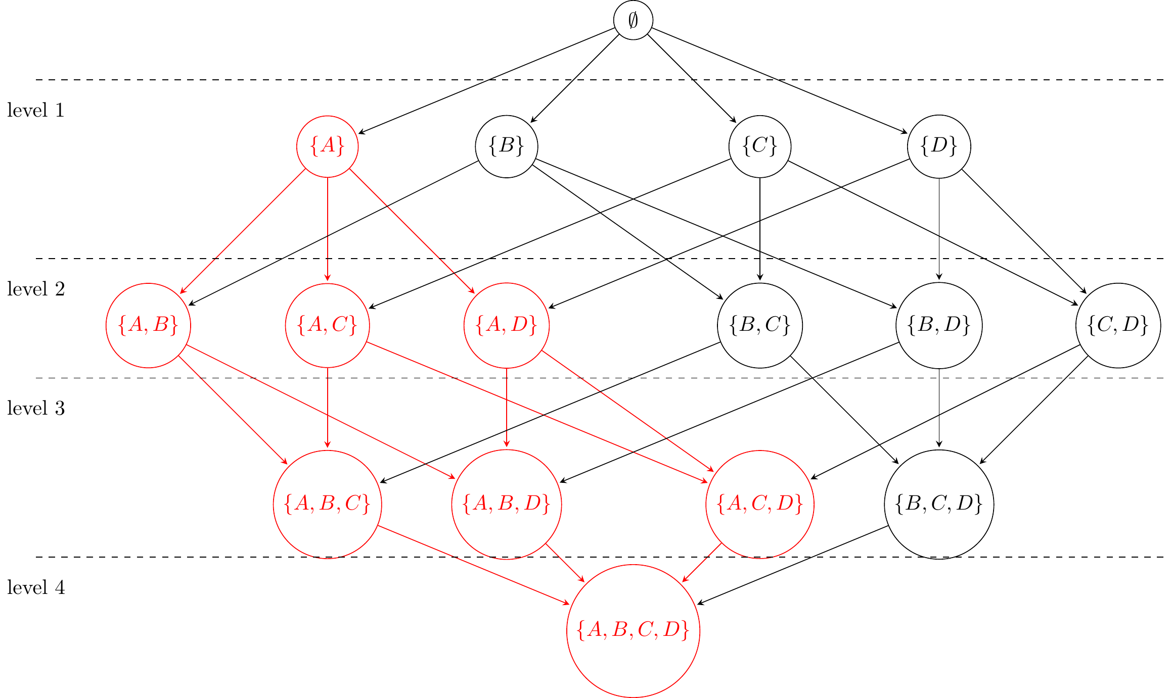
Prune: In this case, we can simplify the search, since if an itemset \(X\) is not frequent, any superset of \(X\) will not be frequent:

For instance, if \(A\) is not frequent we can prune the search space:

One of the earliest (if not the first) algorithm to compute frequent itemsets and association rules is apriori() (implemented in package arules).

It first creates the length 1 itemsets. Remove the infrequent ones (those not obtaining the minimum required support). then, from the _survivors, create length 2 itemsets, and repeat.

6.3.2 Second problem: Association rules

An association rule is a relationship between attributes (items) representing a frequent pattern, i.e. a structural correlation in the table. We denote a rule as \(X\rightarrow Y\). \(X\) is called left hand side or antecedent and \(Y\) is the right hand side or consequent.

Inside of the frequent patterns, we discover the rules.

\[Diapers,Milk, Beer\] is a frequent pattern. What rules are interesting?

For instance, \[Diapers,\, Milk \longrightarrow Beer\] is a rule that can be read “if a person buys diapers and milk, very often he also buys beer”.

Quality of a rule

We have to define some measures of the quality or the interestingness of a rule \(X\rightarrow Y\):

Support: \(Sup(X\rightarrow Y) = Sup(X)\). It is the frequency of the left hand side. A high value indicates that the rule is applicable to a large part of the database. A low value indicates an infrequent rule. Rules with low support may be removed.
Confidence: \(Conf(X\rightarrow Y) = \dfrac{Sup(X\cup Y)}{Sup(X)} = \dfrac{|X\cup Y|}{|X|}\). It is an estimator of \(P(Y|X)\), that is, of the probability in the dataset of having \(Y\) once we know we have \(X\). Indicator of the reliability of the rule.

The confidence of a rule can be very high but the support of the consequent very low. The definition of confidence does not take into account how many times the consequent itemset appears in the table.

Other measures:

Lift: \(Lift(X\rightarrow Y) = \dfrac{Sup(X\cup Y)}{Sup(X)Sup(Y)}\). For a good rule, it should be greater than 1.
Conviction: \(Conv(X\rightarrow Y) = \dfrac{Sup(X)Sup(\overline{Y})}{Sup(X\cup\overline{Y})}\). It approaches 1 as \(X\) and \(Y\) are not related.

But, how do we compute association rules?

There are many possible rules (\(3^{d} - 2^{d+1}+1\), in a dataset with \(d\) items). Instead of using a brute force approach, we begin by using the already computed frequent itemsets.

In addition, we usually set a minimum support and minimum confidence for the extracted rules: this allows to reduce the number of rules to be extracted.

Procedure using A priori:

First, we find all frequent itemsets.

Then, for each itemset found:

Suppose the itemset is \(X = \{x_1, x_2, \ldots, x_n\}\) where \(x_i\) are the different items inside the itemset \(X\).
Consider all rules of the form: \[\{x_1,\ldots,x_{i-1},x_{i+1},\ldots,x_n\}\rightarrow \{x_i\}\]
Compute support and confidence for each rule.
Those rules with less support or confidence are rejected.

Example

Suppose a frequent itemset \(X = \{beer, diapers, milk\}\). We impose a minimum support of 0.4 and minimum confidence of 0.75.

The three possible rules are:

\(\{beer, diapers\}\rightarrow\{milk\}\)
\(\{beer, milk\}\rightarrow\{diapers\}\)
\(\{diapers, milk\}\rightarrow\{beer\}\)

Suppose that we compute their support and confidence in our dataset:

\(Sup(\{beer, diapers\}\rightarrow\{milk\}) = 0.8,\,\, Conf(\{beer, diapers\}\rightarrow\{milk\}) = 0.5\) \(Sup(\{beer, diapers\}\rightarrow\{milk\})=0.3,\,\,Conf(\{beer, diapers\}\rightarrow\{milk\})=0.8\) \(Sup(\{diapers, milk\}\rightarrow\{beer\}) = 0.55,\,\, Conf(\{diapers, milk\}\rightarrow\{beer\}) = 0.9\)

With this information, we reject rules (1) and (2), and store the rule (3), since it verifies the requirements of support and confidence.

6.4 Patterns from binary transactions

Exploring the Adult dataset

library(arules)
data("Adult")
length(Adult)
## [1] 48842
dim(Adult)
## [1] 48842   115
Adult
## transactions in sparse format with
##  48842 transactions (rows) and
##  115 items (columns)
inspect(Adult[1:2])
##     items                                transactionID
## [1] {age=Middle-aged,                                 
##      workclass=State-gov,                             
##      education=Bachelors,                             
##      marital-status=Never-married,                    
##      occupation=Adm-clerical,                         
##      relationship=Not-in-family,                      
##      race=White,                                      
##      sex=Male,                                        
##      capital-gain=Low,                                
##      capital-loss=None,                               
##      hours-per-week=Full-time,                        
##      native-country=United-States,                    
##      income=small}                                   1
## [2] {age=Senior,                                      
##      workclass=Self-emp-not-inc,                      
##      education=Bachelors,                             
##      marital-status=Married-civ-spouse,               
##      occupation=Exec-managerial,                      
##      relationship=Husband,                            
##      race=White,                                      
##      sex=Male,                                        
##      capital-gain=None,                               
##      capital-loss=None,                               
##      hours-per-week=Part-time,                        
##      native-country=United-States,                    
##      income=small}                                   2

To compute the association rules:

data("Adult")
rules <- apriori(Adult, parameter = list(
  supp = 0.5, conf = 0.9,
  target = "frequent itemsets"
))
## Apriori
## 
## Parameter specification:
##  confidence minval smax arem  aval originalSupport maxtime support minlen
##          NA    0.1    1 none FALSE            TRUE       5     0.5      1
##  maxlen            target  ext
##      10 frequent itemsets TRUE
## 
## Algorithmic control:
##  filter tree heap memopt load sort verbose
##     0.1 TRUE TRUE  FALSE TRUE    2    TRUE
## 
## Absolute minimum support count: 24421 
## 
## set item appearances ...[0 item(s)] done [0.00s].
## set transactions ...[115 item(s), 48842 transaction(s)] done [0.02s].
## sorting and recoding items ... [9 item(s)] done [0.00s].
## creating transaction tree ... done [0.01s].
## checking subsets of size 1 2 3 4 done [0.00s].
## sorting transactions ... done [0.00s].
## writing ... [49 set(s)] done [0.00s].
## creating S4 object  ... done [0.00s].

rules <- Adult %>% 
        apriori(parameter = list(
            supp = 0.5, conf = 0.9,
            target = "rules"
))
## Apriori
## 
## Parameter specification:
##  confidence minval smax arem  aval originalSupport maxtime support minlen
##         0.9    0.1    1 none FALSE            TRUE       5     0.5      1
##  maxlen target  ext
##      10  rules TRUE
## 
## Algorithmic control:
##  filter tree heap memopt load sort verbose
##     0.1 TRUE TRUE  FALSE TRUE    2    TRUE
## 
## Absolute minimum support count: 24421 
## 
## set item appearances ...[0 item(s)] done [0.00s].
## set transactions ...[115 item(s), 48842 transaction(s)] done [0.02s].
## sorting and recoding items ... [9 item(s)] done [0.00s].
## creating transaction tree ... done [0.01s].
## checking subsets of size 1 2 3 4 done [0.00s].
## writing ... [52 rule(s)] done [0.00s].
## creating S4 object  ... done [0.00s].

summary(rules)
## set of 52 rules
## 
## rule length distribution (lhs + rhs):sizes
##  1  2  3  4 
##  2 13 24 13 
## 
##    Min. 1st Qu.  Median    Mean 3rd Qu.    Max. 
##   1.000   2.000   3.000   2.923   3.250   4.000 
## 
## summary of quality measures:
##     support         confidence        coverage           lift       
##  Min.   :0.5084   Min.   :0.9031   Min.   :0.5406   Min.   :0.9844  
##  1st Qu.:0.5415   1st Qu.:0.9155   1st Qu.:0.5875   1st Qu.:0.9937  
##  Median :0.5974   Median :0.9229   Median :0.6293   Median :0.9997  
##  Mean   :0.6436   Mean   :0.9308   Mean   :0.6915   Mean   :1.0036  
##  3rd Qu.:0.7426   3rd Qu.:0.9494   3rd Qu.:0.7945   3rd Qu.:1.0057  
##  Max.   :0.9533   Max.   :0.9583   Max.   :1.0000   Max.   :1.0586  
##      count      
##  Min.   :24832  
##  1st Qu.:26447  
##  Median :29178  
##  Mean   :31433  
##  3rd Qu.:36269  
##  Max.   :46560  
## 
## mining info:
##  data ntransactions support confidence
##     .         48842     0.5        0.9
##                                                                           call
##  apriori(data = ., parameter = list(supp = 0.5, conf = 0.9, target = "rules"))
inspect(head(rules))
##     lhs                           rhs                 support   confidence
## [1] {}                         => {capital-gain=None} 0.9173867 0.9173867 
## [2] {}                         => {capital-loss=None} 0.9532779 0.9532779 
## [3] {hours-per-week=Full-time} => {capital-gain=None} 0.5435895 0.9290688 
## [4] {hours-per-week=Full-time} => {capital-loss=None} 0.5606650 0.9582531 
## [5] {sex=Male}                 => {capital-gain=None} 0.6050735 0.9051455 
## [6] {sex=Male}                 => {capital-loss=None} 0.6331027 0.9470750 
##     coverage  lift      count
## [1] 1.0000000 1.0000000 44807
## [2] 1.0000000 1.0000000 46560
## [3] 0.5850907 1.0127342 26550
## [4] 0.5850907 1.0052191 27384
## [5] 0.6684820 0.9866565 29553
## [6] 0.6684820 0.9934931 30922

parameter: list of restrictions on the extraction process

supp or support
conf or confidence
minlen - minimum number of items in itemset
maxlen - maximum number of items in itemset
maxtime - time limit
target - indicate what kind of associations we want to extract: “rules”, “frequent itemsets”, “maximally frequent itemsets”, “closed frequent itemsets”.

rules <- apriori(Adult, parameter = list(supp = 0.1, conf = 1, minlen = 2))
## Apriori
## 
## Parameter specification:
##  confidence minval smax arem  aval originalSupport maxtime support minlen
##           1    0.1    1 none FALSE            TRUE       5     0.1      2
##  maxlen target  ext
##      10  rules TRUE
## 
## Algorithmic control:
##  filter tree heap memopt load sort verbose
##     0.1 TRUE TRUE  FALSE TRUE    2    TRUE
## 
## Absolute minimum support count: 4884 
## 
## set item appearances ...[0 item(s)] done [0.00s].
## set transactions ...[115 item(s), 48842 transaction(s)] done [0.02s].
## sorting and recoding items ... [31 item(s)] done [0.00s].
## creating transaction tree ... done [0.01s].
## checking subsets of size 1 2 3 4 5 6 7 8 9 done [0.05s].
## writing ... [72 rule(s)] done [0.00s].
## creating S4 object  ... done [0.00s].
inspect(tail(rules))
##     lhs                                     rhs          support confidence  coverage     lift count
## [1] {relationship=Husband,                                                                          
##      race=White,                                                                                    
##      capital-gain=None,                                                                             
##      capital-loss=None,                                                                             
##      hours-per-week=Over-time,                                                                      
##      native-country=United-States}       => {sex=Male} 0.1027394          1 0.1027394 1.495926  5018
## [2] {age=Senior,                                                                                    
##      marital-status=Married-civ-spouse,                                                             
##      relationship=Husband,                                                                          
##      race=White,                                                                                    
##      capital-gain=None,                                                                             
##      native-country=United-States}       => {sex=Male} 0.1083698          1 0.1083698 1.495926  5293
## [3] {age=Senior,                                                                                    
##      marital-status=Married-civ-spouse,                                                             
##      relationship=Husband,                                                                          
##      race=White,                                                                                    
##      capital-loss=None,                                                                             
##      native-country=United-States}       => {sex=Male} 0.1167233          1 0.1167233 1.495926  5701
## [4] {age=Senior,                                                                                    
##      marital-status=Married-civ-spouse,                                                             
##      relationship=Husband,                                                                          
##      race=White,                                                                                    
##      capital-gain=None,                                                                             
##      capital-loss=None}                  => {sex=Male} 0.1070800          1 0.1070800 1.495926  5230
## [5] {age=Senior,                                                                                    
##      marital-status=Married-civ-spouse,                                                             
##      relationship=Husband,                                                                          
##      capital-gain=None,                                                                             
##      capital-loss=None,                                                                             
##      native-country=United-States}       => {sex=Male} 0.1072438          1 0.1072438 1.495926  5238
## [6] {marital-status=Married-civ-spouse,                                                             
##      relationship=Husband,                                                                          
##      race=White,                                                                                    
##      capital-gain=None,                                                                             
##      capital-loss=None,                                                                             
##      hours-per-week=Over-time,                                                                      
##      native-country=United-States}       => {sex=Male} 0.1026575          1 0.1026575 1.495926  5014
patterns <- apriori(Adult, parameter = list(supp = 0.5, conf = 0.9, maxlen = 10, target = "frequent itemsets"))
## Apriori
## 
## Parameter specification:
##  confidence minval smax arem  aval originalSupport maxtime support minlen
##          NA    0.1    1 none FALSE            TRUE       5     0.5      1
##  maxlen            target  ext
##      10 frequent itemsets TRUE
## 
## Algorithmic control:
##  filter tree heap memopt load sort verbose
##     0.1 TRUE TRUE  FALSE TRUE    2    TRUE
## 
## Absolute minimum support count: 24421 
## 
## set item appearances ...[0 item(s)] done [0.00s].
## set transactions ...[115 item(s), 48842 transaction(s)] done [0.02s].
## sorting and recoding items ... [9 item(s)] done [0.00s].
## creating transaction tree ... done [0.01s].
## checking subsets of size 1 2 3 4 done [0.00s].
## sorting transactions ... done [0.00s].
## writing ... [49 set(s)] done [0.00s].
## creating S4 object  ... done [0.00s].
summary(patterns)
## set of 49 itemsets
## 
## most frequent items:
##            capital-loss=None            capital-gain=None 
##                           23                           21 
## native-country=United-States                   race=White 
##                           21                           19 
##            workclass=Private                      (Other) 
##                           14                           20 
## 
## element (itemset/transaction) length distribution:sizes
##  1  2  3  4 
##  9 17 17  6 
## 
##    Min. 1st Qu.  Median    Mean 3rd Qu.    Max. 
##   1.000   2.000   2.000   2.408   3.000   4.000 
## 
## summary of quality measures:
##     support           count      
##  Min.   :0.5051   Min.   :24671  
##  1st Qu.:0.5434   1st Qu.:26540  
##  Median :0.5942   Median :29024  
##  Mean   :0.6449   Mean   :31497  
##  3rd Qu.:0.7404   3rd Qu.:36164  
##  Max.   :0.9533   Max.   :46560  
## 
## includes transaction ID lists: FALSE 
## 
## mining info:
##   data ntransactions support confidence
##  Adult         48842     0.5          1
##                                                                                                        call
##  apriori(data = Adult, parameter = list(supp = 0.5, conf = 0.9, maxlen = 10, target = "frequent itemsets"))
inspect(tail(patterns))
##     items                            support count
## [1] {race=White,                                  
##      sex=Male,                                    
##      capital-loss=None,                           
##      native-country=United-States} 0.5113632 24976
## [2] {sex=Male,                                    
##      capital-gain=None,                           
##      capital-loss=None,                           
##      native-country=United-States} 0.5084149 24832
## [3] {workclass=Private,                           
##      race=White,                                  
##      capital-loss=None,                           
##      native-country=United-States} 0.5181401 25307
## [4] {workclass=Private,                           
##      race=White,                                  
##      capital-gain=None,                           
##      capital-loss=None}            0.5204742 25421
## [5] {workclass=Private,                           
##      capital-gain=None,                           
##      capital-loss=None,                           
##      native-country=United-States} 0.5414807 26447
## [6] {race=White,                                  
##      capital-gain=None,                           
##      capital-loss=None,                           
##      native-country=United-States} 0.6803980 33232

appearance: specify restrictions on the extraction of associations.

rules1 <- apriori(Adult,
  parameter = list(supp = 0.1, conf = 0.3),
  appearance = list(rhs = c("relationship=Husband"))
)
## Apriori
## 
## Parameter specification:
##  confidence minval smax arem  aval originalSupport maxtime support minlen
##         0.3    0.1    1 none FALSE            TRUE       5     0.1      1
##  maxlen target  ext
##      10  rules TRUE
## 
## Algorithmic control:
##  filter tree heap memopt load sort verbose
##     0.1 TRUE TRUE  FALSE TRUE    2    TRUE
## 
## Absolute minimum support count: 4884 
## 
## set item appearances ...[1 item(s)] done [0.00s].
## set transactions ...[115 item(s), 48842 transaction(s)] done [0.02s].
## sorting and recoding items ... [31 item(s)] done [0.00s].
## creating transaction tree ... done [0.01s].
## checking subsets of size 1 2 3 4 5 6 7 8 9 done [0.05s].
## writing ... [660 rule(s)] done [0.00s].
## creating S4 object  ... done [0.00s].

inspect(head(rules1))
##     lhs                                    rhs                      support confidence  coverage     lift count
## [1] {}                                  => {relationship=Husband} 0.4036690  0.4036690 1.0000000 1.000000 19716
## [2] {income=large}                      => {relationship=Husband} 0.1211662  0.7547507 0.1605381 1.869727  5918
## [3] {hours-per-week=Over-time}          => {relationship=Husband} 0.1472298  0.5672925 0.2595307 1.405341  7191
## [4] {age=Senior}                        => {relationship=Husband} 0.1479874  0.5673024 0.2608616 1.405365  7228
## [5] {education=HS-grad}                 => {relationship=Husband} 0.1307891  0.4047136 0.3231645 1.002588  6388
## [6] {marital-status=Married-civ-spouse} => {relationship=Husband} 0.4034233  0.8804683 0.4581917 2.181164 19704

rules2 <- apriori(Adult,
  parameter = list(supp = 0.5, conf = 0.9),
  appearance = list(none = c("income=small", "sex=Male"))
)
## Apriori
## 
## Parameter specification:
##  confidence minval smax arem  aval originalSupport maxtime support minlen
##         0.9    0.1    1 none FALSE            TRUE       5     0.5      1
##  maxlen target  ext
##      10  rules TRUE
## 
## Algorithmic control:
##  filter tree heap memopt load sort verbose
##     0.1 TRUE TRUE  FALSE TRUE    2    TRUE
## 
## Absolute minimum support count: 24421 
## 
## set item appearances ...[2 item(s)] done [0.00s].
## set transactions ...[115 item(s), 48842 transaction(s)] done [0.02s].
## sorting and recoding items ... [7 item(s)] done [0.00s].
## creating transaction tree ... done [0.01s].
## checking subsets of size 1 2 3 4 done [0.00s].
## writing ... [39 rule(s)] done [0.00s].
## creating S4 object  ... done [0.00s].

inspect(head(rules2))                             
##     lhs                           rhs                 support   confidence
## [1] {}                         => {capital-gain=None} 0.9173867 0.9173867 
## [2] {}                         => {capital-loss=None} 0.9532779 0.9532779 
## [3] {hours-per-week=Full-time} => {capital-gain=None} 0.5435895 0.9290688 
## [4] {hours-per-week=Full-time} => {capital-loss=None} 0.5606650 0.9582531 
## [5] {workclass=Private}        => {capital-gain=None} 0.6413742 0.9239073 
## [6] {workclass=Private}        => {capital-loss=None} 0.6639982 0.9564974 
##     coverage  lift     count
## [1] 1.0000000 1.000000 44807
## [2] 1.0000000 1.000000 46560
## [3] 0.5850907 1.012734 26550
## [4] 0.5850907 1.005219 27384
## [5] 0.6941976 1.007108 31326
## [6] 0.6941976 1.003377 32431

6.5 Patterns from non binary datasets

Discretize

We are going to explor the AdultUCI dataset. It contains the data from the dataset originally called ‘Census Income’ Database in data.frame format.

The Adult dataset from the previous section has the data prepared for the computation of the rules. The data type of this dataset is transactions which is suitable for the arules package.

The AdultUCI dataset:

library(arules)
data("AdultUCI")
str(AdultUCI)
## 'data.frame':    48842 obs. of  15 variables:
##  $ age           : int  39 50 38 53 28 37 49 52 31 42 ...
##  $ workclass     : Factor w/ 8 levels "Federal-gov",..: 7 6 4 4 4 4 4 6 4 4 ...
##  $ fnlwgt        : int  77516 83311 215646 234721 338409 284582 160187 209642 45781 159449 ...
##  $ education     : Ord.factor w/ 16 levels "Preschool"<"1st-4th"<..: 14 14 9 7 14 15 5 9 15 14 ...
##  $ education-num : int  13 13 9 7 13 14 5 9 14 13 ...
##  $ marital-status: Factor w/ 7 levels "Divorced","Married-AF-spouse",..: 5 3 1 3 3 3 4 3 5 3 ...
##  $ occupation    : Factor w/ 14 levels "Adm-clerical",..: 1 4 6 6 10 4 8 4 10 4 ...
##  $ relationship  : Factor w/ 6 levels "Husband","Not-in-family",..: 2 1 2 1 6 6 2 1 2 1 ...
##  $ race          : Factor w/ 5 levels "Amer-Indian-Eskimo",..: 5 5 5 3 3 5 3 5 5 5 ...
##  $ sex           : Factor w/ 2 levels "Female","Male": 2 2 2 2 1 1 1 2 1 2 ...
##  $ capital-gain  : int  2174 0 0 0 0 0 0 0 14084 5178 ...
##  $ capital-loss  : int  0 0 0 0 0 0 0 0 0 0 ...
##  $ hours-per-week: int  40 13 40 40 40 40 16 45 50 40 ...
##  $ native-country: Factor w/ 41 levels "Cambodia","Canada",..: 39 39 39 39 5 39 23 39 39 39 ...
##  $ income        : Ord.factor w/ 2 levels "small"<"large": 1 1 1 1 1 1 1 2 2 2 ...

For most datasets a first preprocessing step is necessary.

In the following, we will apply preprocessing to AdultUCI until it is converted into transactions that arules handles properly.

Discretisation of items

Delete some columns that are not interesting: fnlwgt, education-num

AdultUCI$fnlwgt <- NULL
## o  AdultUCI[["fnlwgt"]] <- NULL

AdultUCI$`education-num` <- NULL

Convert to discrete numerical values: age, hours-per-week, capital-gain, capital-loss.

We will use cut(), ordered() commands to do this. Here is an example of how these two commands work:

# ejemplo de funcionamiento de cut y ordered
v <- 1:100
v2 <- cut(v, 
          c(0, 25, 50, 75, 100), 
          labels = c("low", "medium", "high", "veryhigh"))
# ?ordered
v3 <- ordered(v2)

We apply these functions to AdultUCI:


AdultUCI$age <- ordered(cut(AdultUCI[["age"]], c(15, 25, 45, 65, 100)),
  labels = c("Young", "Middle-aged", "Senior", "Old")
)

AdultUCI[["hours-per-week"]] <- ordered(cut(
  AdultUCI[["hours-per-week"]],
  c(0, 25, 40, 60, 168)
),
labels = c("Part-time", "Full-time", "Over-time", "Workaholic")
)

AdultUCI[["capital-gain"]] <- ordered(cut(
  AdultUCI[["capital-gain"]],
  c(
    -Inf, 0, median(AdultUCI[["capital-gain"]][AdultUCI[["capital-gain"]] > 0]),
    Inf
  )
), labels = c("None", "Low", "High"))

AdultUCI[["capital-loss"]] <- ordered(cut(
  AdultUCI[["capital-loss"]],
  c(
    -Inf, 0, median(AdultUCI[["capital-loss"]][AdultUCI[["capital-loss"]] > 0]),
    Inf
  )
), labels = c("None", "Low", "High"))

We run apriori():

reg <- apriori(AdultUCI)
## Apriori
## 
## Parameter specification:
##  confidence minval smax arem  aval originalSupport maxtime support minlen
##         0.8    0.1    1 none FALSE            TRUE       5     0.1      1
##  maxlen target  ext
##      10  rules TRUE
## 
## Algorithmic control:
##  filter tree heap memopt load sort verbose
##     0.1 TRUE TRUE  FALSE TRUE    2    TRUE
## 
## Absolute minimum support count: 4884 
## 
## set item appearances ...[0 item(s)] done [0.00s].
## set transactions ...[115 item(s), 48842 transaction(s)] done [0.02s].
## sorting and recoding items ... [31 item(s)] done [0.00s].
## creating transaction tree ... done [0.01s].
## checking subsets of size 1 2 3 4 5 6 7 8 9 done [0.05s].
## writing ... [6137 rule(s)] done [0.00s].
## creating S4 object  ... done [0.00s].
inspect(head(reg))
##     lhs                         rhs                            support  
## [1] {}                       => {race=White}                   0.8550428
## [2] {}                       => {native-country=United-States} 0.8974243
## [3] {}                       => {capital-gain=None}            0.9173867
## [4] {}                       => {capital-loss=None}            0.9532779
## [5] {relationship=Unmarried} => {capital-loss=None}            0.1019819
## [6] {occupation=Sales}       => {race=White}                   0.1005282
##     confidence coverage  lift     count
## [1] 0.8550428  1.0000000 1.000000 41762
## [2] 0.8974243  1.0000000 1.000000 43832
## [3] 0.9173867  1.0000000 1.000000 44807
## [4] 0.9532779  1.0000000 1.000000 46560
## [5] 0.9719024  0.1049302 1.019537  4981
## [6] 0.8920785  0.1126899 1.043314  4910

See this link.

We compare AdultUCI that we have processed with Adult..

Adult1 <- as(AdultUCI, "transactions")
class(Adult1)
## [1] "transactions"
## attr(,"package")
## [1] "arules"
length(Adult1)
## [1] 48842
dim(Adult1)
## [1] 48842   115
Adult1
## transactions in sparse format with
##  48842 transactions (rows) and
##  115 items (columns)
inspect(Adult1[1:2])
##     items                                transactionID
## [1] {age=Middle-aged,                                 
##      workclass=State-gov,                             
##      education=Bachelors,                             
##      marital-status=Never-married,                    
##      occupation=Adm-clerical,                         
##      relationship=Not-in-family,                      
##      race=White,                                      
##      sex=Male,                                        
##      capital-gain=Low,                                
##      capital-loss=None,                               
##      hours-per-week=Full-time,                        
##      native-country=United-States,                    
##      income=small}                                   1
## [2] {age=Senior,                                      
##      workclass=Self-emp-not-inc,                      
##      education=Bachelors,                             
##      marital-status=Married-civ-spouse,               
##      occupation=Exec-managerial,                      
##      relationship=Husband,                            
##      race=White,                                      
##      sex=Male,                                        
##      capital-gain=None,                               
##      capital-loss=None,                               
##      hours-per-week=Part-time,                        
##      native-country=United-States,                    
##      income=small}                                   2

data("Adult")
class(Adult)
## [1] "transactions"
## attr(,"package")
## [1] "arules"
length(Adult)
## [1] 48842
dim(Adult)
## [1] 48842   115
Adult
## transactions in sparse format with
##  48842 transactions (rows) and
##  115 items (columns)
inspect(Adult[1:2])
##     items                                transactionID
## [1] {age=Middle-aged,                                 
##      workclass=State-gov,                             
##      education=Bachelors,                             
##      marital-status=Never-married,                    
##      occupation=Adm-clerical,                         
##      relationship=Not-in-family,                      
##      race=White,                                      
##      sex=Male,                                        
##      capital-gain=Low,                                
##      capital-loss=None,                               
##      hours-per-week=Full-time,                        
##      native-country=United-States,                    
##      income=small}                                   1
## [2] {age=Senior,                                      
##      workclass=Self-emp-not-inc,                      
##      education=Bachelors,                             
##      marital-status=Married-civ-spouse,               
##      occupation=Exec-managerial,                      
##      relationship=Husband,                            
##      race=White,                                      
##      sex=Male,                                        
##      capital-gain=None,                               
##      capital-loss=None,                               
##      hours-per-week=Part-time,                        
##      native-country=United-States,                    
##      income=small}                                   2

6.6 Methods of `arules` package.

summary(): Overview of the set of rules.
length(): Number of rules.
items(): Items involved.
sort(): Sort
subset(): Items involved. (see help(subset)). Select rules that meet certain criteria.
union(), intersect(), setequal(), match() (use help(xxx)).
write(): Writing more properly formatted rules.

Operations with rules:

data("Adult")
r1 <- apriori(Adult[1:1000], parameter = list(support = 0.5))
r2 <- apriori(Adult[1001:2000], parameter = list(support = 0.5))
# Convertir en un dataframe
dfr1 <- DATAFRAME(r1)
r_comb <- c(r1, r2)
duplicated(r_comb)
intersect(r1, r2)
union(r1, r2)
lhs(reglas1)
rhs(reglas1)
class(lhs(reglas1))

6.7 `arulesViz` package

Let’s use the Groceries dataset to look at the most interesting association rule display commands.

We extract the rules:

library(arules)
library(arulesViz)
data(Groceries)
rules <- apriori(Groceries, parameter = list(support = 0.001, confidence = 0.5))
## Apriori
## 
## Parameter specification:
##  confidence minval smax arem  aval originalSupport maxtime support minlen
##         0.5    0.1    1 none FALSE            TRUE       5   0.001      1
##  maxlen target  ext
##      10  rules TRUE
## 
## Algorithmic control:
##  filter tree heap memopt load sort verbose
##     0.1 TRUE TRUE  FALSE TRUE    2    TRUE
## 
## Absolute minimum support count: 9 
## 
## set item appearances ...[0 item(s)] done [0.00s].
## set transactions ...[169 item(s), 9835 transaction(s)] done [0.00s].
## sorting and recoding items ... [157 item(s)] done [0.00s].
## creating transaction tree ... done [0.00s].
## checking subsets of size 1 2 3 4 5 6 done [0.01s].
## writing ... [5668 rule(s)] done [0.00s].
## creating S4 object  ... done [0.00s].
rules
## set of 5668 rules
inspect(head(rules))
##     lhs                    rhs          support     confidence coverage   
## [1] {honey}             => {whole milk} 0.001118454 0.7333333  0.001525165
## [2] {tidbits}           => {rolls/buns} 0.001220132 0.5217391  0.002338587
## [3] {cocoa drinks}      => {whole milk} 0.001321810 0.5909091  0.002236909
## [4] {pudding powder}    => {whole milk} 0.001321810 0.5652174  0.002338587
## [5] {cooking chocolate} => {whole milk} 0.001321810 0.5200000  0.002541942
## [6] {cereals}           => {whole milk} 0.003660397 0.6428571  0.005693950
##     lift     count
## [1] 2.870009 11   
## [2] 2.836542 12   
## [3] 2.312611 13   
## [4] 2.212062 13   
## [5] 2.035097 13   
## [6] 2.515917 36

The basic rule visualisation command is plot(). We show different options for using plot() (colours).

plot(rules)
## To reduce overplotting, jitter is added! Use jitter = 0 to prevent jitter.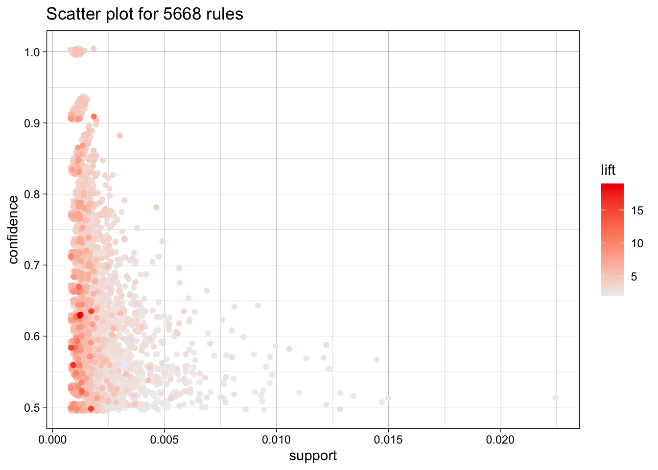

library(colorspace)
plot(rules, control = list(col = sequential_hcl(100)))
## To reduce overplotting, jitter is added! Use jitter = 0 to prevent jitter.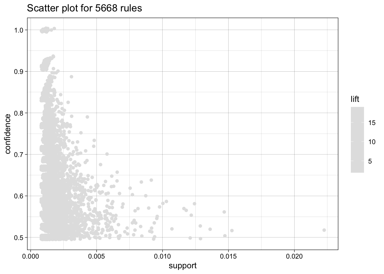

plot(rules, col = sequential_hcl(100))
## To reduce overplotting, jitter is added! Use jitter = 0 to prevent jitter.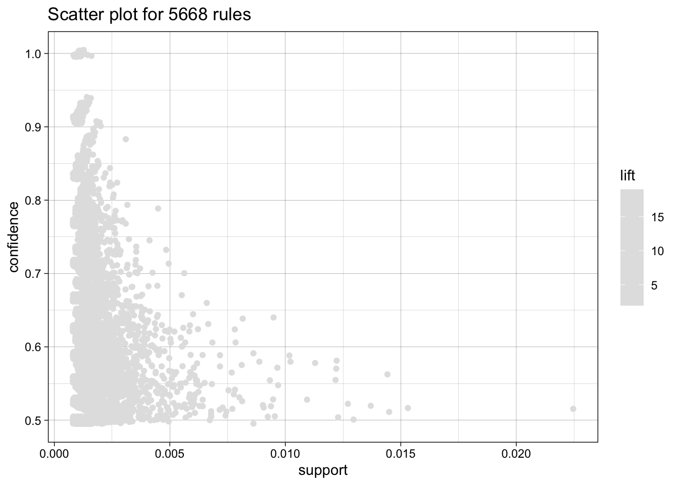

plot(rules, col = grey.colors(50, alpha = .8))
## To reduce overplotting, jitter is added! Use jitter = 0 to prevent jitter.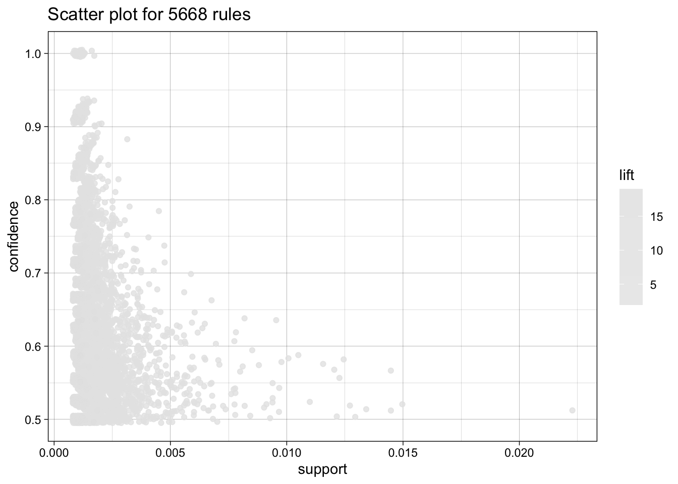

Interactive display option:

# Ejecutar en vuestro ordenador
sel <- plot(rules, engine = "interactive")
plot(rules, engine = "htmlwidget")

Matrix representation of rules:

subrules <- subset(rules, lift > 8)
subrules
## set of 52 rules
plot(subrules, method = "matrix")
## Itemsets in Antecedent (LHS)
##  [1] "{Instant food products,soda}"                                              
##  [2] "{soda,popcorn}"                                                            
##  [3] "{flour,baking powder}"                                                     
##  [4] "{ham,processed cheese}"                                                    
##  [5] "{whole milk,Instant food products}"                                        
##  [6] "{other vegetables,curd,yogurt,whipped/sour cream}"                         
##  [7] "{processed cheese,domestic eggs}"                                          
##  [8] "{tropical fruit,other vegetables,yogurt,white bread}"                      
##  [9] "{hamburger meat,yogurt,whipped/sour cream}"                                
## [10] "{tropical fruit,other vegetables,whole milk,yogurt,domestic eggs}"         
## [11] "{liquor,red/blush wine}"                                                   
## [12] "{other vegetables,yogurt,whipped/sour cream,cream cheese }"                
## [13] "{yogurt,whipped/sour cream,hard cheese}"                                   
## [14] "{tropical fruit,root vegetables,other vegetables,whole milk,rolls/buns}"   
## [15] "{tropical fruit,whole milk,yogurt,sliced cheese}"                          
## [16] "{other vegetables,butter,sugar}"                                           
## [17] "{whole milk,whipped/sour cream,hard cheese}"                               
## [18] "{other vegetables,hard cheese,domestic eggs}"                              
## [19] "{tropical fruit,other vegetables,whipped/sour cream,fruit/vegetable juice}"
## [20] "{tropical fruit,onions,yogurt}"                                            
## [21] "{tropical fruit,other vegetables,yogurt,domestic eggs}"                    
## [22] "{butter,yogurt,pastry}"                                                    
## [23] "{whole milk,butter,hard cheese}"                                           
## [24] "{tropical fruit,other vegetables,butter,fruit/vegetable juice}"            
## [25] "{whole milk,curd,yogurt,cream cheese }"                                    
## [26] "{tropical fruit,other vegetables,hard cheese}"                             
## [27] "{other vegetables,whole milk,whipped/sour cream,napkins}"                  
## [28] "{citrus fruit,whole milk,cream cheese }"                                   
## [29] "{tropical fruit,other vegetables,frozen fish}"                             
## [30] "{butter,yogurt,hard cheese}"                                               
## [31] "{curd,yogurt,sugar}"                                                       
## [32] "{other vegetables,whole milk,butter,soda}"                                 
## [33] "{whole milk,cream cheese ,sugar}"                                          
## [34] "{frozen vegetables,specialty chocolate}"                                   
## [35] "{citrus fruit,other vegetables,whole milk,cream cheese }"                  
## [36] "{tropical fruit,whipped/sour cream,shopping bags}"                         
## [37] "{citrus fruit,tropical fruit,grapes}"                                      
## [38] "{other vegetables,butter,hard cheese}"                                     
## [39] "{whole milk,butter,sliced cheese}"                                         
## [40] "{citrus fruit,other vegetables,soda,fruit/vegetable juice}"                
## [41] "{tropical fruit,other vegetables,whole milk,yogurt,oil}"                   
## [42] "{tropical fruit,grapes,fruit/vegetable juice}"                             
## [43] "{frankfurter,tropical fruit,domestic eggs}"                                
## [44] "{tropical fruit,whole milk,yogurt,frozen meals}"                           
## [45] "{other vegetables,curd,yogurt,cream cheese }"                              
## [46] "{root vegetables,whole milk,flour}"                                        
## [47] "{citrus fruit,whole milk,sugar}"                                           
## [48] "{tropical fruit,other vegetables,misc. beverages}"                         
## [49] "{ham,tropical fruit,other vegetables}"                                     
## [50] "{citrus fruit,grapes,fruit/vegetable juice}"                               
## [51] "{whole milk,whipped/sour cream,rolls/buns,pastry}"                         
## Itemsets in Consequent (RHS)
##  [1] "{tropical fruit}"        "{citrus fruit}"         
##  [3] "{root vegetables}"       "{pip fruit}"            
##  [5] "{fruit/vegetable juice}" "{domestic eggs}"        
##  [7] "{whipped/sour cream}"    "{butter}"               
##  [9] "{curd}"                  "{beef}"                 
## [11] "{bottled beer}"          "{white bread}"          
## [13] "{cream cheese }"         "{sugar}"                
## [15] "{salty snack}"           "{hamburger meat}"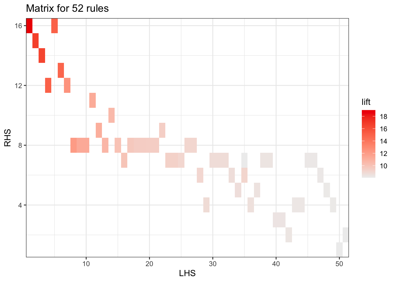

plot(subrules, method = "matrix", engine = "3d")
## Itemsets in Antecedent (LHS)
##  [1] "{Instant food products,soda}"                                              
##  [2] "{soda,popcorn}"                                                            
##  [3] "{flour,baking powder}"                                                     
##  [4] "{ham,processed cheese}"                                                    
##  [5] "{whole milk,Instant food products}"                                        
##  [6] "{other vegetables,curd,yogurt,whipped/sour cream}"                         
##  [7] "{processed cheese,domestic eggs}"                                          
##  [8] "{tropical fruit,other vegetables,yogurt,white bread}"                      
##  [9] "{hamburger meat,yogurt,whipped/sour cream}"                                
## [10] "{tropical fruit,other vegetables,whole milk,yogurt,domestic eggs}"         
## [11] "{liquor,red/blush wine}"                                                   
## [12] "{other vegetables,yogurt,whipped/sour cream,cream cheese }"                
## [13] "{yogurt,whipped/sour cream,hard cheese}"                                   
## [14] "{tropical fruit,root vegetables,other vegetables,whole milk,rolls/buns}"   
## [15] "{tropical fruit,whole milk,yogurt,sliced cheese}"                          
## [16] "{other vegetables,butter,sugar}"                                           
## [17] "{whole milk,whipped/sour cream,hard cheese}"                               
## [18] "{other vegetables,hard cheese,domestic eggs}"                              
## [19] "{tropical fruit,other vegetables,whipped/sour cream,fruit/vegetable juice}"
## [20] "{tropical fruit,onions,yogurt}"                                            
## [21] "{tropical fruit,other vegetables,yogurt,domestic eggs}"                    
## [22] "{butter,yogurt,pastry}"                                                    
## [23] "{whole milk,butter,hard cheese}"                                           
## [24] "{tropical fruit,other vegetables,butter,fruit/vegetable juice}"            
## [25] "{whole milk,curd,yogurt,cream cheese }"                                    
## [26] "{tropical fruit,other vegetables,hard cheese}"                             
## [27] "{other vegetables,whole milk,whipped/sour cream,napkins}"                  
## [28] "{citrus fruit,whole milk,cream cheese }"                                   
## [29] "{tropical fruit,other vegetables,frozen fish}"                             
## [30] "{butter,yogurt,hard cheese}"                                               
## [31] "{curd,yogurt,sugar}"                                                       
## [32] "{other vegetables,whole milk,butter,soda}"                                 
## [33] "{whole milk,cream cheese ,sugar}"                                          
## [34] "{frozen vegetables,specialty chocolate}"                                   
## [35] "{citrus fruit,other vegetables,whole milk,cream cheese }"                  
## [36] "{tropical fruit,whipped/sour cream,shopping bags}"                         
## [37] "{citrus fruit,tropical fruit,grapes}"                                      
## [38] "{other vegetables,butter,hard cheese}"                                     
## [39] "{whole milk,butter,sliced cheese}"                                         
## [40] "{citrus fruit,other vegetables,soda,fruit/vegetable juice}"                
## [41] "{tropical fruit,other vegetables,whole milk,yogurt,oil}"                   
## [42] "{tropical fruit,grapes,fruit/vegetable juice}"                             
## [43] "{frankfurter,tropical fruit,domestic eggs}"                                
## [44] "{tropical fruit,whole milk,yogurt,frozen meals}"                           
## [45] "{other vegetables,curd,yogurt,cream cheese }"                              
## [46] "{root vegetables,whole milk,flour}"                                        
## [47] "{citrus fruit,whole milk,sugar}"                                           
## [48] "{tropical fruit,other vegetables,misc. beverages}"                         
## [49] "{ham,tropical fruit,other vegetables}"                                     
## [50] "{citrus fruit,grapes,fruit/vegetable juice}"                               
## [51] "{whole milk,whipped/sour cream,rolls/buns,pastry}"                         
## Itemsets in Consequent (RHS)
##  [1] "{tropical fruit}"        "{citrus fruit}"         
##  [3] "{root vegetables}"       "{pip fruit}"            
##  [5] "{fruit/vegetable juice}" "{domestic eggs}"        
##  [7] "{whipped/sour cream}"    "{butter}"               
##  [9] "{curd}"                  "{beef}"                 
## [11] "{bottled beer}"          "{white bread}"          
## [13] "{cream cheese }"         "{sugar}"                
## [15] "{salty snack}"           "{hamburger meat}"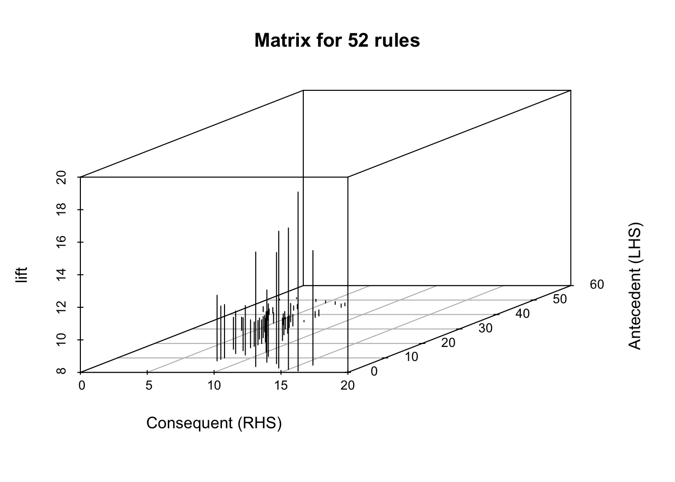

plot(subrules, method = "matrix", 
     measure = "lift",
     shading = "confidence")
## Itemsets in Antecedent (LHS)
##  [1] "{citrus fruit,other vegetables,soda,fruit/vegetable juice}"                
##  [2] "{tropical fruit,other vegetables,whole milk,yogurt,oil}"                   
##  [3] "{liquor,red/blush wine}"                                                   
##  [4] "{citrus fruit,grapes,fruit/vegetable juice}"                               
##  [5] "{other vegetables,butter,sugar}"                                           
##  [6] "{tropical fruit,grapes,fruit/vegetable juice}"                             
##  [7] "{tropical fruit,other vegetables,frozen fish}"                             
##  [8] "{whole milk,butter,hard cheese}"                                           
##  [9] "{tropical fruit,other vegetables,yogurt,white bread}"                      
## [10] "{tropical fruit,other vegetables,butter,fruit/vegetable juice}"            
## [11] "{whole milk,whipped/sour cream,rolls/buns,pastry}"                         
## [12] "{tropical fruit,whipped/sour cream,shopping bags}"                         
## [13] "{whole milk,curd,yogurt,cream cheese }"                                    
## [14] "{ham,processed cheese}"                                                    
## [15] "{soda,popcorn}"                                                            
## [16] "{Instant food products,soda}"                                              
## [17] "{frozen vegetables,specialty chocolate}"                                   
## [18] "{butter,yogurt,hard cheese}"                                               
## [19] "{hamburger meat,yogurt,whipped/sour cream}"                                
## [20] "{curd,yogurt,sugar}"                                                       
## [21] "{frankfurter,tropical fruit,domestic eggs}"                                
## [22] "{tropical fruit,whole milk,yogurt,frozen meals}"                           
## [23] "{other vegetables,whole milk,butter,soda}"                                 
## [24] "{tropical fruit,other vegetables,whole milk,yogurt,domestic eggs}"         
## [25] "{ham,tropical fruit,other vegetables}"                                     
## [26] "{citrus fruit,tropical fruit,grapes}"                                      
## [27] "{other vegetables,butter,hard cheese}"                                     
## [28] "{whole milk,butter,sliced cheese}"                                         
## [29] "{tropical fruit,other vegetables,misc. beverages}"                         
## [30] "{yogurt,whipped/sour cream,hard cheese}"                                   
## [31] "{other vegetables,curd,yogurt,cream cheese }"                              
## [32] "{other vegetables,yogurt,whipped/sour cream,cream cheese }"                
## [33] "{other vegetables,curd,yogurt,whipped/sour cream}"                         
## [34] "{root vegetables,whole milk,flour}"                                        
## [35] "{citrus fruit,other vegetables,whole milk,cream cheese }"                  
## [36] "{citrus fruit,whole milk,cream cheese }"                                   
## [37] "{flour,baking powder}"                                                     
## [38] "{tropical fruit,whole milk,yogurt,sliced cheese}"                          
## [39] "{whole milk,cream cheese ,sugar}"                                          
## [40] "{tropical fruit,root vegetables,other vegetables,whole milk,rolls/buns}"   
## [41] "{whole milk,whipped/sour cream,hard cheese}"                               
## [42] "{other vegetables,hard cheese,domestic eggs}"                              
## [43] "{tropical fruit,other vegetables,whipped/sour cream,fruit/vegetable juice}"
## [44] "{processed cheese,domestic eggs}"                                          
## [45] "{tropical fruit,onions,yogurt}"                                            
## [46] "{tropical fruit,other vegetables,yogurt,domestic eggs}"                    
## [47] "{citrus fruit,whole milk,sugar}"                                           
## [48] "{whole milk,Instant food products}"                                        
## [49] "{tropical fruit,other vegetables,hard cheese}"                             
## [50] "{butter,yogurt,pastry}"                                                    
## [51] "{other vegetables,whole milk,whipped/sour cream,napkins}"                  
## Itemsets in Consequent (RHS)
##  [1] "{curd}"                  "{beef}"                 
##  [3] "{domestic eggs}"         "{sugar}"                
##  [5] "{butter}"                "{hamburger meat}"       
##  [7] "{white bread}"           "{cream cheese }"        
##  [9] "{fruit/vegetable juice}" "{whipped/sour cream}"   
## [11] "{salty snack}"           "{pip fruit}"            
## [13] "{citrus fruit}"          "{tropical fruit}"       
## [15] "{bottled beer}"          "{root vegetables}"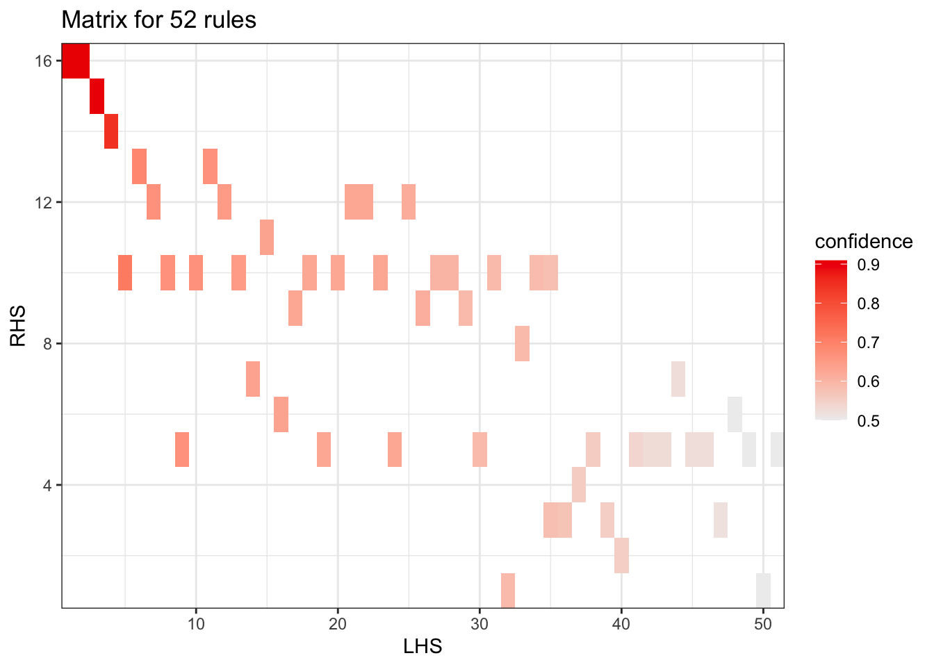

And interactive:

# Ejecutar en vuestro ordenador
plot(subrules, method = "matrix", engine = "interactive")
plot(subrules, method = "matrix", engine = "htmlwidget")

Matrix representation showing the items:

# Ejecutar en vuestro ordenador
plot(subrules, method = "grouped matrix")
plot(subrules,
  method = "grouped matrix",
  col = grey.colors(10),
  gp_labels = gpar(col = "blue", cex = 1, fontface = "italic")
)
# sel <- plot(rules, method="grouped", engine = "interactive")

Network representation of rules (only for small sets of rules):

subrules2 <- sample(subrules, 5)
plot(subrules2, method = "graph")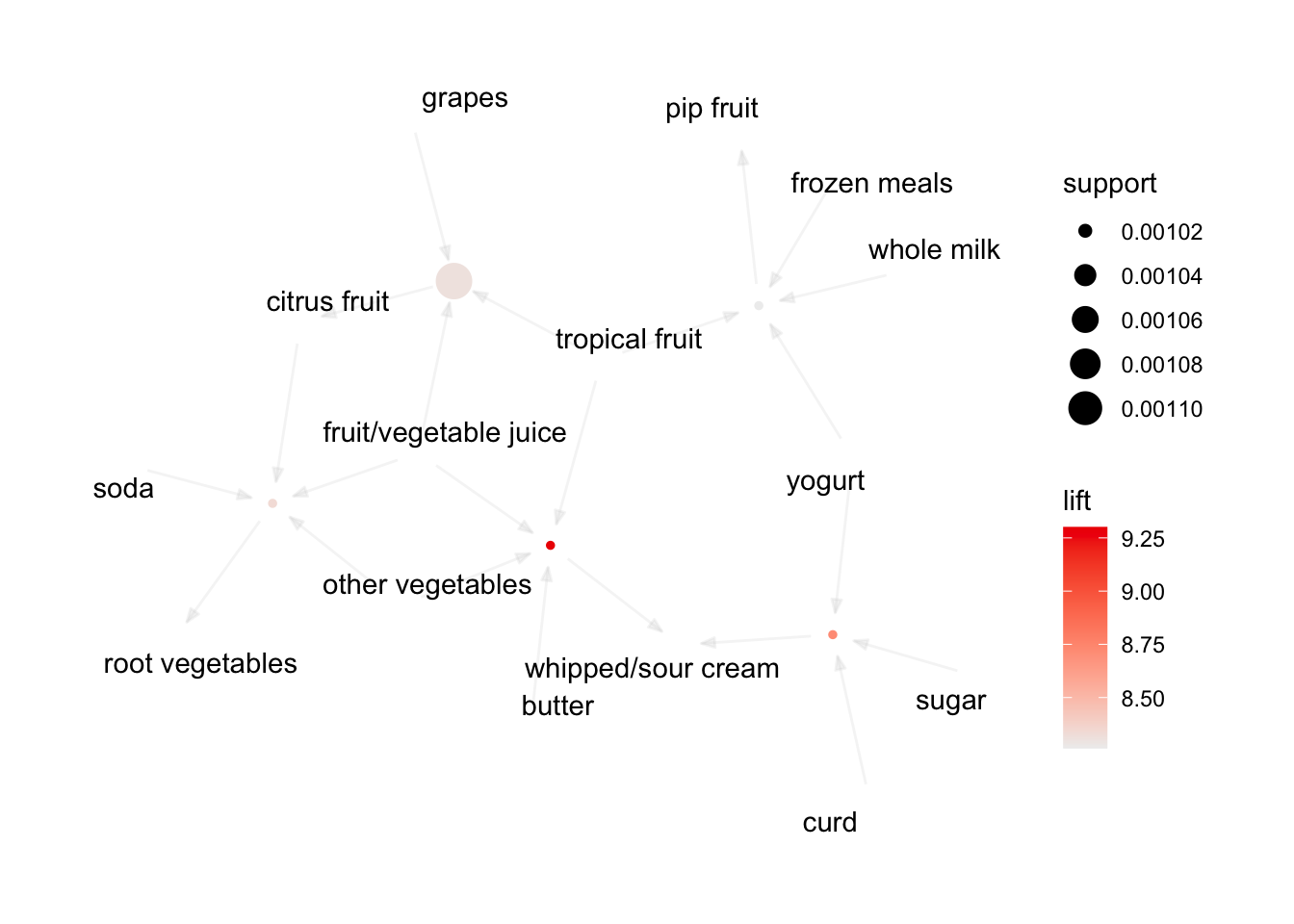

plot(subrules2,
  method = "graph",
  nodeCol = grey.colors(10), edgeCol = grey(.7), alpha = 1
)
## Warning: Unknown control parameters: nodeCol, edgeCol, alpha
## Available control parameters (with default values):
## layout    =  stress
## circular  =  FALSE
## ggraphdots    =  NULL
## edges     =  <environment>
## nodes     =  <environment>
## nodetext  =  <environment>
## colors    =  c("#EE0000FF", "#EEEEEEFF")
## engine    =  ggplot2
## max   =  100
## verbose   =  FALSE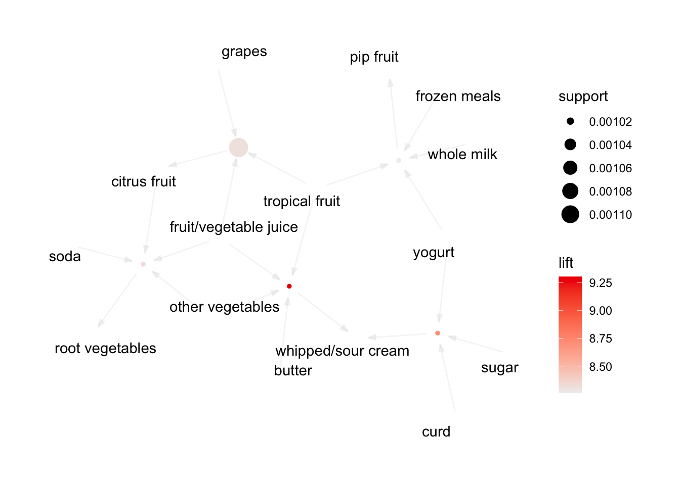

The Graphviz package allows for better visualisation:

plot(subrules2, method = "graph", engine = "graphviz")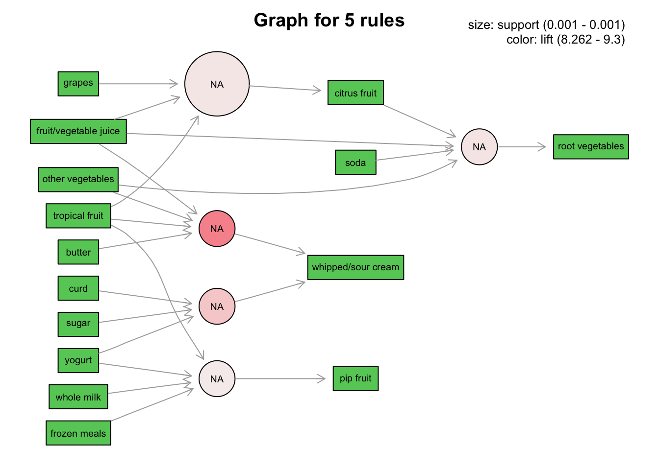

It allows dynamic visualisation:

# Ejecutar en local
plot(subrules2, method = "graph", engine = "htmlwidget")
plot(subrules2,
  method = "graph", engine = "htmlwidget",
  igraphLayout = "layout_in_circle"
)

6.8 A recommender system

Analysis of relationships between songs

The lastfm.csv dataset includes transactions collected from an online radio station that stores user ID, artist, user gender and country.

Objective: To build a system for recommending music groups to users from the above dataset.

library(arules)
lastfm <- read.csv("lastfm.csv")
lastfm[1:20, ]
##    user                  artist sex       country
## 1     1   red hot chili peppers   f       Germany
## 2     1 the black dahlia murder   f       Germany
## 3     1               goldfrapp   f       Germany
## 4     1        dropkick murphys   f       Germany
## 5     1                le tigre   f       Germany
## 6     1              schandmaul   f       Germany
## 7     1                   edguy   f       Germany
## 8     1            jack johnson   f       Germany
## 9     1               eluveitie   f       Germany
## 10    1             the killers   f       Germany
## 11    1            judas priest   f       Germany
## 12    1              rob zombie   f       Germany
## 13    1              john mayer   f       Germany
## 14    1                 the who   f       Germany
## 15    1              guano apes   f       Germany
## 16    1      the rolling stones   f       Germany
## 17    3        devendra banhart   m United States
## 18    3        boards of canada   m United States
## 19    3               cocorosie   m United States
## 20    3              aphex twin   m United States
length(lastfm$user) ## 289,955 filas
## [1] 289955
class(lastfm$user)
## [1] "integer"
# We need to convert this attribute to a factor in order to be able to analyse it with package {"arules"}.

lastfm$user <- factor(lastfm$user)
# Run on your computer
# levels(lastfm$user)  ## 15,000 users
# levels(lastfm$artist)  ## 1,004 artists

We call apriori():

reglas1 <- apriori(lastfm, parameter = list(support = .01, confidence = .5))
## Warning: Column(s) 2, 3, 4 not logical or factor. Applying default
## discretization (see '? discretizeDF').
## Apriori
## 
## Parameter specification:
##  confidence minval smax arem  aval originalSupport maxtime support minlen
##         0.5    0.1    1 none FALSE            TRUE       5    0.01      1
##  maxlen target  ext
##      10  rules TRUE
## 
## Algorithmic control:
##  filter tree heap memopt load sort verbose
##     0.1 TRUE TRUE  FALSE TRUE    2    TRUE
## 
## Absolute minimum support count: 2899 
## 
## set item appearances ...[0 item(s)] done [0.00s].
## set transactions ...[16165 item(s), 289955 transaction(s)] done [0.13s].
## sorting and recoding items ... [21 item(s)] done [0.00s].
## creating transaction tree ... done [0.03s].
## checking subsets of size 1 2 done [0.00s].
## writing ... [19 rule(s)] done [0.00s].
## creating S4 object  ... done [0.01s].
inspect(reglas1)
##      lhs                             rhs     support    confidence coverage  
## [1]  {}                           => {sex=m} 0.73053750 0.7305375  1.00000000
## [2]  {country=Czech Republic}     => {sex=m} 0.01039472 0.8033049  0.01293994
## [3]  {country=Mexico}             => {sex=m} 0.01023607 0.7804365  0.01311583
## [4]  {country=Norway}             => {sex=m} 0.01239503 0.7744021  0.01600593
## [5]  {country=Turkey}             => {sex=m} 0.01088445 0.6627467  0.01642324
## [6]  {country=Italy}              => {sex=m} 0.01501612 0.7615882  0.01971685
## [7]  {country=France}             => {sex=m} 0.01707161 0.8302583  0.02056181
## [8]  {country=Australia}          => {sex=m} 0.01497474 0.6776963  0.02209653
## [9]  {country=Canada}             => {sex=m} 0.01568174 0.6563222  0.02389336
## [10] {country=Spain}              => {sex=m} 0.02482109 0.7720446  0.03214982
## [11] {country=Netherlands}        => {sex=m} 0.02690417 0.8064716  0.03336035
## [12] {country=Finland}            => {sex=m} 0.02661103 0.7596731  0.03502957
## [13] {country=Russian Federation} => {sex=m} 0.03062544 0.7605344  0.04026832
## [14] {country=Brazil}             => {sex=m} 0.03001845 0.7300788  0.04111673
## [15] {country=Sweden}             => {sex=m} 0.03193254 0.7479603  0.04269283
## [16] {country=Poland}             => {sex=m} 0.03854391 0.6531471  0.05901261
## [17] {country=Germany}            => {sex=m} 0.06069907 0.7257433  0.08363712
## [18] {country=United Kingdom}     => {sex=m} 0.07730510 0.8110211  0.09531824
## [19] {country=United States}      => {sex=m} 0.13852839 0.6744182  0.20540429
##      lift      count 
## [1]  1.0000000 211823
## [2]  1.0996080   3014
## [3]  1.0683045   2968
## [4]  1.0600442   3594
## [5]  0.9072043   3156
## [6]  1.0425040   4354
## [7]  1.1365033   4950
## [8]  0.9276680   4342
## [9]  0.8984100   4547
## [10] 1.0568172   7197
## [11] 1.1039428   7801
## [12] 1.0398825   7716
## [13] 1.0410615   8880
## [14] 0.9993722   8704
## [15] 1.0238492   9259
## [16] 0.8940638  11176
## [17] 0.9934374  17600
## [18] 1.1101703  22415
## [19] 0.9231808  40167

Comment: In previous versions of arules the previous command gave an error. We had to convert discrete variables to factor. It is a live package that is evolving day by day.

**What is the recommendation we can get with these rules?

It is not the kind of rules we want to get for our recommender system.

Rules for making recommendations

The data must be manipulated in order to find what we are interested in. We will use the commands: split(), lapply().

First I keep a list of what each user listens to:

lista.musica.por.usuario <- split(x = lastfm[, "artist"], f = lastfm$user)
lista.musica.por.usuario[1:2]
## $`1`
##  [1] "red hot chili peppers"   "the black dahlia murder"
##  [3] "goldfrapp"               "dropkick murphys"       
##  [5] "le tigre"                "schandmaul"             
##  [7] "edguy"                   "jack johnson"           
##  [9] "eluveitie"               "the killers"            
## [11] "judas priest"            "rob zombie"             
## [13] "john mayer"              "the who"                
## [15] "guano apes"              "the rolling stones"     
## 
## $`3`
##  [1] "devendra banhart"    "boards of canada"    "cocorosie"          
##  [4] "aphex twin"          "animal collective"   "atmosphere"         
##  [7] "joanna newsom"       "air"                 "portishead"         
## [10] "massive attack"      "broken social scene" "arcade fire"        
## [13] "plaid"               "prefuse 73"          "m83"                
## [16] "the flashbulb"       "pavement"            "goldfrapp"          
## [19] "amon tobin"          "sage francis"        "four tet"           
## [22] "max richter"         "autechre"            "radiohead"          
## [25] "neutral milk hotel"  "beastie boys"        "aesop rock"         
## [28] "mf doom"             "the books"

A group/singer could be in a user twice: remove repeats
Convert to transaction format
Look at the music listened to by the first users

## Remove duplicates
lista.musica.por.usuario <- lapply(lista.musica.por.usuario, unique)

# We convert the music list into transactions.
lista.musica.por.usuario1 <- as(lista.musica.por.usuario, "transactions")

lista.musica.por.usuario[1:5]
## $`1`
##  [1] "red hot chili peppers"   "the black dahlia murder"
##  [3] "goldfrapp"               "dropkick murphys"       
##  [5] "le tigre"                "schandmaul"             
##  [7] "edguy"                   "jack johnson"           
##  [9] "eluveitie"               "the killers"            
## [11] "judas priest"            "rob zombie"             
## [13] "john mayer"              "the who"                
## [15] "guano apes"              "the rolling stones"     
## 
## $`3`
##  [1] "devendra banhart"    "boards of canada"    "cocorosie"          
##  [4] "aphex twin"          "animal collective"   "atmosphere"         
##  [7] "joanna newsom"       "air"                 "portishead"         
## [10] "massive attack"      "broken social scene" "arcade fire"        
## [13] "plaid"               "prefuse 73"          "m83"                
## [16] "the flashbulb"       "pavement"            "goldfrapp"          
## [19] "amon tobin"          "sage francis"        "four tet"           
## [22] "max richter"         "autechre"            "radiohead"          
## [25] "neutral milk hotel"  "beastie boys"        "aesop rock"         
## [28] "mf doom"             "the books"          
## 
## $`4`
##  [1] "tv on the radio"         "tool"                   
##  [3] "kyuss"                   "dj shadow"              
##  [5] "air"                     "a tribe called quest"   
##  [7] "the cinematic orchestra" "beck"                   
##  [9] "bon iver"                "röyksopp"               
## [11] "bonobo"                  "the decemberists"       
## [13] "snow patrol"             "battles"                
## [15] "the prodigy"             "pink floyd"             
## [17] "rjd2"                    "the flaming lips"       
## [19] "michael jackson"         "mgmt"                   
## [21] "the rolling stones"      "late of the pier"       
## [23] "flight of the conchords" "simian mobile disco"    
## [25] "muse"                    "fleetwood mac"          
## [27] "led zeppelin"           
## 
## $`5`
##  [1] "dream theater"            "ac/dc"                   
##  [3] "metallica"                "iron maiden"             
##  [5] "bob marley & the wailers" "megadeth"                
##  [7] "children of bodom"        "trivium"                 
##  [9] "nightwish"                "sublime"                 
## [11] "volbeat"                 
## 
## $`6`
##  [1] "lily allen"           "kanye west"           "sigur rós"           
##  [4] "pink floyd"           "stevie wonder"        "metallica"           
##  [7] "thievery corporation" "iron maiden"          "the streets"         
## [10] "muse"                 "faith no more"        "manu chao"           
## [13] "tenacious d"          "depeche mode"         "justin timberlake"   
## [16] "green day"            "snow patrol"          "dream theater"       
## [19] "u2"                   "jay-z"                "type o negative"     
## [22] "pearl jam"            "queen"

We visualise what we have achieved so far:

str(lista.musica.por.usuario1)
## Formal class 'transactions' [package "arules"] with 3 slots
##   ..@ data       :Formal class 'ngCMatrix' [package "Matrix"] with 5 slots
##   .. .. ..@ i       : int [1:289953] 280 288 299 373 383 429 457 468 512 714 ...
##   .. .. ..@ p       : int [1:15001] 0 16 45 72 83 106 128 147 177 184 ...
##   .. .. ..@ Dim     : int [1:2] 1004 15000
##   .. .. ..@ Dimnames:List of 2
##   .. .. .. ..$ : NULL
##   .. .. .. ..$ : NULL
##   .. .. ..@ factors : list()
##   ..@ itemInfo   :'data.frame':  1004 obs. of  1 variable:
##   .. ..$ labels: chr [1:1004] "...and you will know us by the trail of dead" "[unknown]" "2pac" "3 doors down" ...
##   ..@ itemsetInfo:'data.frame':  15000 obs. of  1 variable:
##   .. ..$ transactionID: chr [1:15000] "1" "3" "4" "5" ...
write(head(lista.musica.por.usuario1))
## "dropkick murphys" "edguy" "eluveitie" "goldfrapp" "guano apes" "jack johnson" "john mayer" "judas priest" "le tigre" "red hot chili peppers" "rob zombie" "schandmaul" "the black dahlia murder" "the killers" "the rolling stones" "the who"
## "aesop rock" "air" "amon tobin" "animal collective" "aphex twin" "arcade fire" "atmosphere" "autechre" "beastie boys" "boards of canada" "broken social scene" "cocorosie" "devendra banhart" "four tet" "goldfrapp" "joanna newsom" "m83" "massive attack" "max richter" "mf doom" "neutral milk hotel" "pavement" "plaid" "portishead" "prefuse 73" "radiohead" "sage francis" "the books" "the flashbulb"
## "a tribe called quest" "air" "battles" "beck" "bon iver" "bonobo" "dj shadow" "fleetwood mac" "flight of the conchords" "kyuss" "late of the pier" "led zeppelin" "mgmt" "michael jackson" "muse" "pink floyd" "rjd2" "röyksopp" "simian mobile disco" "snow patrol" "the cinematic orchestra" "the decemberists" "the flaming lips" "the prodigy" "the rolling stones" "tool" "tv on the radio"
## "ac/dc" "bob marley & the wailers" "children of bodom" "dream theater" "iron maiden" "megadeth" "metallica" "nightwish" "sublime" "trivium" "volbeat"
## "depeche mode" "dream theater" "faith no more" "green day" "iron maiden" "jay-z" "justin timberlake" "kanye west" "lily allen" "manu chao" "metallica" "muse" "pearl jam" "pink floyd" "queen" "sigur rós" "snow patrol" "stevie wonder" "tenacious d" "the streets" "thievery corporation" "type o negative" "u2"
## "ac/dc" "aerosmith" "alice in chains" "audioslave" "buckethead" "camel" "disturbed" "dream theater" "jethro tull" "king crimson" "led zeppelin" "oasis" "pearl jam" "pink floyd" "porcupine tree" "rammstein" "rush" "soundgarden" "stone temple pilots" "the verve" "tool" "type o negative"
write(head(lista.musica.por.usuario1), format = "single")
## "1" "dropkick murphys"
## "1" "edguy"
## "1" "eluveitie"
## "1" "goldfrapp"
## "1" "guano apes"
## "1" "jack johnson"
## "1" "john mayer"
## "1" "judas priest"
## "1" "le tigre"
## "1" "red hot chili peppers"
## "1" "rob zombie"
## "1" "schandmaul"
## "1" "the black dahlia murder"
## "1" "the killers"
## "1" "the rolling stones"
## "1" "the who"
## "3" "aesop rock"
## "3" "air"
## "3" "amon tobin"
## "3" "animal collective"
## "3" "aphex twin"
## "3" "arcade fire"
## "3" "atmosphere"
## "3" "autechre"
## "3" "beastie boys"
## "3" "boards of canada"
## "3" "broken social scene"
## "3" "cocorosie"
## "3" "devendra banhart"
## "3" "four tet"
## "3" "goldfrapp"
## "3" "joanna newsom"
## "3" "m83"
## "3" "massive attack"
## "3" "max richter"
## "3" "mf doom"
## "3" "neutral milk hotel"
## "3" "pavement"
## "3" "plaid"
## "3" "portishead"
## "3" "prefuse 73"
## "3" "radiohead"
## "3" "sage francis"
## "3" "the books"
## "3" "the flashbulb"
## "4" "a tribe called quest"
## "4" "air"
## "4" "battles"
## "4" "beck"
## "4" "bon iver"
## "4" "bonobo"
## "4" "dj shadow"
## "4" "fleetwood mac"
## "4" "flight of the conchords"
## "4" "kyuss"
## "4" "late of the pier"
## "4" "led zeppelin"
## "4" "mgmt"
## "4" "michael jackson"
## "4" "muse"
## "4" "pink floyd"
## "4" "rjd2"
## "4" "röyksopp"
## "4" "simian mobile disco"
## "4" "snow patrol"
## "4" "the cinematic orchestra"
## "4" "the decemberists"
## "4" "the flaming lips"
## "4" "the prodigy"
## "4" "the rolling stones"
## "4" "tool"
## "4" "tv on the radio"
## "5" "ac/dc"
## "5" "bob marley & the wailers"
## "5" "children of bodom"
## "5" "dream theater"
## "5" "iron maiden"
## "5" "megadeth"
## "5" "metallica"
## "5" "nightwish"
## "5" "sublime"
## "5" "trivium"
## "5" "volbeat"
## "6" "depeche mode"
## "6" "dream theater"
## "6" "faith no more"
## "6" "green day"
## "6" "iron maiden"
## "6" "jay-z"
## "6" "justin timberlake"
## "6" "kanye west"
## "6" "lily allen"
## "6" "manu chao"
## "6" "metallica"
## "6" "muse"
## "6" "pearl jam"
## "6" "pink floyd"
## "6" "queen"
## "6" "sigur rós"
## "6" "snow patrol"
## "6" "stevie wonder"
## "6" "tenacious d"
## "6" "the streets"
## "6" "thievery corporation"
## "6" "type o negative"
## "6" "u2"
## "7" "ac/dc"
## "7" "aerosmith"
## "7" "alice in chains"
## "7" "audioslave"
## "7" "buckethead"
## "7" "camel"
## "7" "disturbed"
## "7" "dream theater"
## "7" "jethro tull"
## "7" "king crimson"
## "7" "led zeppelin"
## "7" "oasis"
## "7" "pearl jam"
## "7" "pink floyd"
## "7" "porcupine tree"
## "7" "rammstein"
## "7" "rush"
## "7" "soundgarden"
## "7" "stone temple pilots"
## "7" "the verve"
## "7" "tool"
## "7" "type o negative"

It is a list of transactions - data type defined in arules. We calculate the relative frequency of the songs listened to:

itfreq1 <- itemFrequency(lista.musica.por.usuario1)
head(itfreq1)
## ...and you will know us by the trail of dead 
##                                  0.009800000 
##                                    [unknown] 
##                                  0.036866667 
##                                         2pac 
##                                  0.022733333 
##                                 3 doors down 
##                                  0.030933333 
##                           30 seconds to mars 
##                                  0.032800000 
##                                          311 
##                                  0.008333333

itfreq1:

is a numeric vector
the names of the list (names(itfreq) — the names of each group )
each position therefore is the frequency of the group of that position

Draw the frequencies using the list of transactions obtained:

itemFrequencyPlot(lista.musica.por.usuario1, support = .1, cex.names = 1)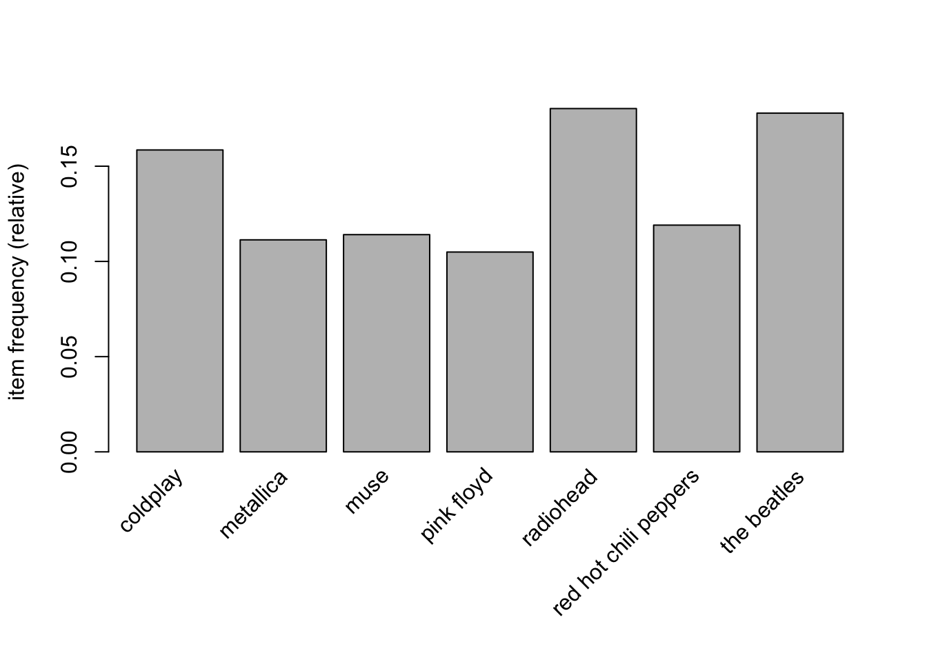

And we obtain the association rules with support 0.1 and confidence 0.5:

reglas2 <- apriori(lista.musica.por.usuario1,
  parameter =
    list(support = .01, confidence = .5)
)
## Apriori
## 
## Parameter specification:
##  confidence minval smax arem  aval originalSupport maxtime support minlen
##         0.5    0.1    1 none FALSE            TRUE       5    0.01      1
##  maxlen target  ext
##      10  rules TRUE
## 
## Algorithmic control:
##  filter tree heap memopt load sort verbose
##     0.1 TRUE TRUE  FALSE TRUE    2    TRUE
## 
## Absolute minimum support count: 150 
## 
## set item appearances ...[0 item(s)] done [0.00s].
## set transactions ...[1004 item(s), 15000 transaction(s)] done [0.02s].
## sorting and recoding items ... [655 item(s)] done [0.00s].
## creating transaction tree ... done [0.00s].
## checking subsets of size 1 2 3 4 done [0.01s].
## writing ... [50 rule(s)] done [0.00s].
## creating S4 object  ... done [0.00s].
reglas2
## set of 50 rules
inspect(reglas2)
##      lhs                                     rhs            support   
## [1]  {t.i.}                               => {kanye west}   0.01040000
## [2]  {the pussycat dolls}                 => {rihanna}      0.01040000
## [3]  {the fray}                           => {coldplay}     0.01126667
## [4]  {sonata arctica}                     => {nightwish}    0.01346667
## [5]  {judas priest}                       => {iron maiden}  0.01353333
## [6]  {the kinks}                          => {the beatles}  0.01360000
## [7]  {travis}                             => {coldplay}     0.01373333
## [8]  {the flaming lips}                   => {radiohead}    0.01306667
## [9]  {megadeth}                           => {metallica}    0.01626667
## [10] {simon & garfunkel}                  => {the beatles}  0.01540000
## [11] {broken social scene}                => {radiohead}    0.01506667
## [12] {blur}                               => {radiohead}    0.01753333
## [13] {keane}                              => {coldplay}     0.02226667
## [14] {snow patrol}                        => {coldplay}     0.02646667
## [15] {beck}                               => {radiohead}    0.02926667
## [16] {snow patrol, the killers}           => {coldplay}     0.01040000
## [17] {radiohead, snow patrol}             => {coldplay}     0.01006667
## [18] {death cab for cutie, the shins}     => {radiohead}    0.01006667
## [19] {the beatles, the shins}             => {radiohead}    0.01066667
## [20] {led zeppelin, the doors}            => {pink floyd}   0.01066667
## [21] {pink floyd, the doors}              => {led zeppelin} 0.01066667
## [22] {pink floyd, the doors}              => {the beatles}  0.01000000
## [23] {the beatles, the strokes}           => {radiohead}    0.01046667
## [24] {oasis, the killers}                 => {coldplay}     0.01113333
## [25] {oasis, the beatles}                 => {coldplay}     0.01060000
## [26] {oasis, radiohead}                   => {coldplay}     0.01273333
## [27] {beck, the beatles}                  => {radiohead}    0.01300000
## [28] {bob dylan, the rolling stones}      => {the beatles}  0.01146667
## [29] {david bowie, the rolling stones}    => {the beatles}  0.01000000
## [30] {led zeppelin, the rolling stones}   => {the beatles}  0.01066667
## [31] {radiohead, the rolling stones}      => {the beatles}  0.01060000
## [32] {coldplay, the smashing pumpkins}    => {radiohead}    0.01093333
## [33] {the beatles, the smashing pumpkins} => {radiohead}    0.01146667
## [34] {radiohead, u2}                      => {coldplay}     0.01140000
## [35] {coldplay, sigur rós}                => {radiohead}    0.01206667
## [36] {sigur rós, the beatles}             => {radiohead}    0.01046667
## [37] {bob dylan, pink floyd}              => {the beatles}  0.01033333
## [38] {bob dylan, radiohead}               => {the beatles}  0.01386667
## [39] {bloc party, the killers}            => {coldplay}     0.01106667
## [40] {david bowie, pink floyd}            => {the beatles}  0.01006667
## [41] {david bowie, radiohead}             => {the beatles}  0.01393333
## [42] {placebo, radiohead}                 => {muse}         0.01366667
## [43] {led zeppelin, radiohead}            => {the beatles}  0.01306667
## [44] {death cab for cutie, the killers}   => {coldplay}     0.01086667
## [45] {death cab for cutie, the beatles}   => {radiohead}    0.01246667
## [46] {muse, the killers}                  => {coldplay}     0.01513333
## [47] {red hot chili peppers, the killers} => {coldplay}     0.01086667
## [48] {the beatles, the killers}           => {coldplay}     0.01253333
## [49] {radiohead, the killers}             => {coldplay}     0.01506667
## [50] {muse, the beatles}                  => {radiohead}    0.01380000
##      confidence coverage   lift      count
## [1]  0.5672727  0.01833333  8.854413 156  
## [2]  0.5777778  0.01800000 13.415893 156  
## [3]  0.5168196  0.02180000  3.260006 169  
## [4]  0.5101010  0.02640000  8.236292 202  
## [5]  0.5075000  0.02666667  8.562992 203  
## [6]  0.5298701  0.02566667  2.979030 204  
## [7]  0.5628415  0.02440000  3.550304 206  
## [8]  0.5297297  0.02466667  2.938589 196  
## [9]  0.5281385  0.03080000  4.743759 244  
## [10] 0.5238095  0.02940000  2.944956 231  
## [11] 0.5472155  0.02753333  3.035589 226  
## [12] 0.5228628  0.03353333  2.900496 263  
## [13] 0.6374046  0.03493333  4.020634 334  
## [14] 0.5251323  0.05040000  3.312441 397  
## [15] 0.5092807  0.05746667  2.825152 439  
## [16] 0.5954198  0.01746667  3.755802 156  
## [17] 0.6344538  0.01586667  4.002021 151  
## [18] 0.5033333  0.02000000  2.792160 151  
## [19] 0.5673759  0.01880000  3.147425 160  
## [20] 0.5970149  0.01786667  5.689469 160  
## [21] 0.5387205  0.01980000  6.802027 160  
## [22] 0.5050505  0.01980000  2.839489 150  
## [23] 0.5607143  0.01866667  3.110471 157  
## [24] 0.6626984  0.01680000  4.180183 167  
## [25] 0.5196078  0.02040000  3.277594 159  
## [26] 0.5876923  0.02166667  3.707058 191  
## [27] 0.5909091  0.02200000  3.277972 195  
## [28] 0.5910653  0.01940000  3.323081 172  
## [29] 0.5703422  0.01753333  3.206572 150  
## [30] 0.5776173  0.01846667  3.247474 160  
## [31] 0.5638298  0.01880000  3.169958 159  
## [32] 0.6283525  0.01740000  3.485683 164  
## [33] 0.6209386  0.01846667  3.444556 172  
## [34] 0.5213415  0.02186667  3.288529 171  
## [35] 0.5801282  0.02080000  3.218167 181  
## [36] 0.6434426  0.01626667  3.569393 157  
## [37] 0.6150794  0.01680000  3.458092 155  
## [38] 0.5730028  0.02420000  3.221530 208  
## [39] 0.5236593  0.02113333  3.303150 166  
## [40] 0.5741445  0.01753333  3.227949 151  
## [41] 0.5225000  0.02666667  2.937594 209  
## [42] 0.5137845  0.02660000  4.504247 205  
## [43] 0.5283019  0.02473333  2.970213 196  
## [44] 0.5884477  0.01846667  3.711823 163  
## [45] 0.5013405  0.02486667  2.781105 187  
## [46] 0.5089686  0.02973333  3.210483 227  
## [47] 0.5093750  0.02133333  3.213047 163  
## [48] 0.5340909  0.02346667  3.368950 188  
## [49] 0.5243619  0.02873333  3.307582 226  
## [50] 0.5073529  0.02720000  2.814458 207

Recommendation system

First we keep the most interesting rules. We filter out those with lift greater than 1:

inspect(subset(reglas2, subset = lift > 3.5))
##      lhs                                   rhs            support    confidence
## [1]  {t.i.}                             => {kanye west}   0.01040000 0.5672727 
## [2]  {the pussycat dolls}               => {rihanna}      0.01040000 0.5777778 
## [3]  {sonata arctica}                   => {nightwish}    0.01346667 0.5101010 
## [4]  {judas priest}                     => {iron maiden}  0.01353333 0.5075000 
## [5]  {travis}                           => {coldplay}     0.01373333 0.5628415 
## [6]  {megadeth}                         => {metallica}    0.01626667 0.5281385 
## [7]  {keane}                            => {coldplay}     0.02226667 0.6374046 
## [8]  {snow patrol, the killers}         => {coldplay}     0.01040000 0.5954198 
## [9]  {radiohead, snow patrol}           => {coldplay}     0.01006667 0.6344538 
## [10] {led zeppelin, the doors}          => {pink floyd}   0.01066667 0.5970149 
## [11] {pink floyd, the doors}            => {led zeppelin} 0.01066667 0.5387205 
## [12] {oasis, the killers}               => {coldplay}     0.01113333 0.6626984 
## [13] {oasis, radiohead}                 => {coldplay}     0.01273333 0.5876923 
## [14] {sigur rós, the beatles}           => {radiohead}    0.01046667 0.6434426 
## [15] {placebo, radiohead}               => {muse}         0.01366667 0.5137845 
## [16] {death cab for cutie, the killers} => {coldplay}     0.01086667 0.5884477 
##      coverage   lift      count
## [1]  0.01833333  8.854413 156  
## [2]  0.01800000 13.415893 156  
## [3]  0.02640000  8.236292 202  
## [4]  0.02666667  8.562992 203  
## [5]  0.02440000  3.550304 206  
## [6]  0.03080000  4.743759 244  
## [7]  0.03493333  4.020634 334  
## [8]  0.01746667  3.755802 156  
## [9]  0.01586667  4.002021 151  
## [10] 0.01786667  5.689469 160  
## [11] 0.01980000  6.802027 160  
## [12] 0.01680000  4.180183 167  
## [13] 0.02166667  3.707058 191  
## [14] 0.01626667  3.569393 157  
## [15] 0.02660000  4.504247 205  
## [16] 0.01846667  3.711823 163

We order by confidence these rules above:

inspect(sort(subset(reglas2, subset = lift > 1), by = "confidence"))
##      lhs                                     rhs            support   
## [1]  {oasis, the killers}                 => {coldplay}     0.01113333
## [2]  {sigur rós, the beatles}             => {radiohead}    0.01046667
## [3]  {keane}                              => {coldplay}     0.02226667
## [4]  {radiohead, snow patrol}             => {coldplay}     0.01006667
## [5]  {coldplay, the smashing pumpkins}    => {radiohead}    0.01093333
## [6]  {the beatles, the smashing pumpkins} => {radiohead}    0.01146667
## [7]  {bob dylan, pink floyd}              => {the beatles}  0.01033333
## [8]  {led zeppelin, the doors}            => {pink floyd}   0.01066667
## [9]  {snow patrol, the killers}           => {coldplay}     0.01040000
## [10] {bob dylan, the rolling stones}      => {the beatles}  0.01146667
## [11] {beck, the beatles}                  => {radiohead}    0.01300000
## [12] {death cab for cutie, the killers}   => {coldplay}     0.01086667
## [13] {oasis, radiohead}                   => {coldplay}     0.01273333
## [14] {coldplay, sigur rós}                => {radiohead}    0.01206667
## [15] {the pussycat dolls}                 => {rihanna}      0.01040000
## [16] {led zeppelin, the rolling stones}   => {the beatles}  0.01066667
## [17] {david bowie, pink floyd}            => {the beatles}  0.01006667
## [18] {bob dylan, radiohead}               => {the beatles}  0.01386667
## [19] {david bowie, the rolling stones}    => {the beatles}  0.01000000
## [20] {the beatles, the shins}             => {radiohead}    0.01066667
## [21] {t.i.}                               => {kanye west}   0.01040000
## [22] {radiohead, the rolling stones}      => {the beatles}  0.01060000
## [23] {travis}                             => {coldplay}     0.01373333
## [24] {the beatles, the strokes}           => {radiohead}    0.01046667
## [25] {broken social scene}                => {radiohead}    0.01506667
## [26] {pink floyd, the doors}              => {led zeppelin} 0.01066667
## [27] {the beatles, the killers}           => {coldplay}     0.01253333
## [28] {the kinks}                          => {the beatles}  0.01360000
## [29] {the flaming lips}                   => {radiohead}    0.01306667
## [30] {led zeppelin, radiohead}            => {the beatles}  0.01306667
## [31] {megadeth}                           => {metallica}    0.01626667
## [32] {snow patrol}                        => {coldplay}     0.02646667
## [33] {radiohead, the killers}             => {coldplay}     0.01506667
## [34] {simon & garfunkel}                  => {the beatles}  0.01540000
## [35] {bloc party, the killers}            => {coldplay}     0.01106667
## [36] {blur}                               => {radiohead}    0.01753333
## [37] {david bowie, radiohead}             => {the beatles}  0.01393333
## [38] {radiohead, u2}                      => {coldplay}     0.01140000
## [39] {oasis, the beatles}                 => {coldplay}     0.01060000
## [40] {the fray}                           => {coldplay}     0.01126667
## [41] {placebo, radiohead}                 => {muse}         0.01366667
## [42] {sonata arctica}                     => {nightwish}    0.01346667
## [43] {red hot chili peppers, the killers} => {coldplay}     0.01086667
## [44] {beck}                               => {radiohead}    0.02926667
## [45] {muse, the killers}                  => {coldplay}     0.01513333
## [46] {judas priest}                       => {iron maiden}  0.01353333
## [47] {muse, the beatles}                  => {radiohead}    0.01380000
## [48] {pink floyd, the doors}              => {the beatles}  0.01000000
## [49] {death cab for cutie, the shins}     => {radiohead}    0.01006667
## [50] {death cab for cutie, the beatles}   => {radiohead}    0.01246667
##      confidence coverage   lift      count
## [1]  0.6626984  0.01680000  4.180183 167  
## [2]  0.6434426  0.01626667  3.569393 157  
## [3]  0.6374046  0.03493333  4.020634 334  
## [4]  0.6344538  0.01586667  4.002021 151  
## [5]  0.6283525  0.01740000  3.485683 164  
## [6]  0.6209386  0.01846667  3.444556 172  
## [7]  0.6150794  0.01680000  3.458092 155  
## [8]  0.5970149  0.01786667  5.689469 160  
## [9]  0.5954198  0.01746667  3.755802 156  
## [10] 0.5910653  0.01940000  3.323081 172  
## [11] 0.5909091  0.02200000  3.277972 195  
## [12] 0.5884477  0.01846667  3.711823 163  
## [13] 0.5876923  0.02166667  3.707058 191  
## [14] 0.5801282  0.02080000  3.218167 181  
## [15] 0.5777778  0.01800000 13.415893 156  
## [16] 0.5776173  0.01846667  3.247474 160  
## [17] 0.5741445  0.01753333  3.227949 151  
## [18] 0.5730028  0.02420000  3.221530 208  
## [19] 0.5703422  0.01753333  3.206572 150  
## [20] 0.5673759  0.01880000  3.147425 160  
## [21] 0.5672727  0.01833333  8.854413 156  
## [22] 0.5638298  0.01880000  3.169958 159  
## [23] 0.5628415  0.02440000  3.550304 206  
## [24] 0.5607143  0.01866667  3.110471 157  
## [25] 0.5472155  0.02753333  3.035589 226  
## [26] 0.5387205  0.01980000  6.802027 160  
## [27] 0.5340909  0.02346667  3.368950 188  
## [28] 0.5298701  0.02566667  2.979030 204  
## [29] 0.5297297  0.02466667  2.938589 196  
## [30] 0.5283019  0.02473333  2.970213 196  
## [31] 0.5281385  0.03080000  4.743759 244  
## [32] 0.5251323  0.05040000  3.312441 397  
## [33] 0.5243619  0.02873333  3.307582 226  
## [34] 0.5238095  0.02940000  2.944956 231  
## [35] 0.5236593  0.02113333  3.303150 166  
## [36] 0.5228628  0.03353333  2.900496 263  
## [37] 0.5225000  0.02666667  2.937594 209  
## [38] 0.5213415  0.02186667  3.288529 171  
## [39] 0.5196078  0.02040000  3.277594 159  
## [40] 0.5168196  0.02180000  3.260006 169  
## [41] 0.5137845  0.02660000  4.504247 205  
## [42] 0.5101010  0.02640000  8.236292 202  
## [43] 0.5093750  0.02133333  3.213047 163  
## [44] 0.5092807  0.05746667  2.825152 439  
## [45] 0.5089686  0.02973333  3.210483 227  
## [46] 0.5075000  0.02666667  8.562992 203  
## [47] 0.5073529  0.02720000  2.814458 207  
## [48] 0.5050505  0.01980000  2.839489 150  
## [49] 0.5033333  0.02000000  2.792160 151  
## [50] 0.5013405  0.02486667  2.781105 187

Recommendation to users who listen to Coldplay?:

r1 <- subset(reglas2, subset = lhs %pin%
  c("cold"))
inspect(r1)
##     lhs                                  rhs         support    confidence
## [1] {coldplay, the smashing pumpkins} => {radiohead} 0.01093333 0.6283525 
## [2] {coldplay, sigur rós}             => {radiohead} 0.01206667 0.5801282 
##     coverage lift     count
## [1] 0.0174   3.485683 164  
## [2] 0.0208   3.218167 181

Try other groups.