# Example in R
data <- c(5, 8, 3, 10, 5, 6)
mean(data)
## [1] 6.1666671 Preliminaries
In this section, we recall some fundamental concepts in statistics, which are essential for understanding data and its characteristics. This is not intended to be an exhaustive dictionary of terms and theoretical results, just a reminder of some ideas and concepts that a student should possess by the time he/she starts the Master.
1.1 Descriptive Statistics
Descriptive statistics provide simple summaries of the data and form the foundation for further analysis. They help to describe, show, or summarize data in a meaningful way. Below, we explore key measures:
1.1.1 Central Tendency Measures
These metrics indicate the central point around which the data is distributed.
The mean is the arithmetic average, calculated as the sum of all observations divided by the number of observations. It is calculated as:
\[ \bar{x} = \frac{1}{n} \sum_{i=1}^{n} x_i \]
The median is the middle value of a data set when it is ordered from least to greatest. If the number of observations is even, it is the average of the two middle numbers.
median(data)
## [1] 5.5
The mode is the value that appears most frequently in the data set. A data set may have more than one mode.
# Using the mode function to find the most frequent value
getmode <- function(v) {
   uniqv <- unique(v)
   uniqv[which.max(tabulate(match(v, uniqv)))]
}
getmode(data)
## [1] 5
Quartiles divide the data into four equal parts, each representing 25% of the data points. There are three quartiles:
- Q1 (First Quartile): The value below which 25% of the data falls.
- Q2 (Second Quartile or Median): The value below which 50% of the data falls.
- Q3 (Third Quartile): The value below which 75% of the data falls.
Quartiles provide a robust way of understanding the spread of data without being affected by extreme values, making them especially useful when comparing distributions.
\[ Q_1 = \text{25th percentile}, \quad Q_2 = \text{50th percentile (Median)}, \quad Q_3 = \text{75th percentile} \]
quantile(data)
##   0%  25%  50%  75% 100%
##  3.0  5.0  5.5  7.5 10.0
1.1.2 Statistical Dispersion Measures
Dispersion metrics quantify the spread or variability of the data, indicating how spread out the values are.
Variance is the average of the squared differences from the mean. It provides insight into the degree of spread in the data:
\[ \mathrm{var}(X) = \sigma^2 = \frac{1}{n} \sum_{i=1}^{n} (x_i - \bar{x})^2 \]
var(data)
## [1] 6.166667
The standard deviation measures the amount of variation or dispersion in a data set. It is the square root of the variance:
\[ \sigma = \sqrt{\frac{1}{n} \sum_{i=1}^{n} (x_i - \bar{x})^2} \]
sd(data)
## [1] 2.483277
The Interquartile range (IQR) is a measure of statistical dispersion, representing the range within which the central 50% of values fall. It is the difference between the third quartile (Q3) and the first quartile (Q1):
\[ \mathrm{IQR} = Q_3 - Q_1 \]
IQR(data)
## [1] 2.5
The range is the difference between the maximum and minimum values in the dataset:
\[ \mathrm{Range} = \max(x) - \min(x) \]
range(data)
## [1]  3 10
1.1.3 Other Measures
Skewness quantifies the asymmetry of the probability distribution of a real-valued random variable about its mean. Positive skew indicates that the right tail is longer, while negative skew indicates that the left tail is longer.
\[ \mathrm{Skewness} = \frac{n}{(n-1)(n-2)} \sum_{i=1}^{n} \left( \frac{x_i - \bar{x}}{s} \right)^3 \]
library(e1071) # We need another library
## Warning: package 'e1071' was built under R version 4.3.3
skewness(data)
## [1] 0.299904
Kurtosis measures the “tailedness” of the probability distribution. High kurtosis indicates heavy tails, while low kurtosis indicates light tails compared to a normal distribution.
\[ \mathrm{Kurtosis} = \frac{n(n+1)}{(n-1)(n-2)(n-3)} \sum_{i=1}^{n} \left( \frac{x_i - \bar{x}}{s} \right)^4 - \frac{3(n-1)^2}{(n-2)(n-3)} \]
kurtosis(data)
## [1] -1.547176
1.1.4 Visualizing Descriptive Statistics
Visualizations are an essential part of descriptive statistics. Below, we create visualizations for the data, including a histogram, boxplot, and density plot. These help to visually assess the central tendency, spread, skewness, and potential outliers in the dataset.
A histogram shows the distribution of a dataset by plotting the frequency of data points in discrete intervals (bins).
hist(data,
     main = "Histogram of Data",
     xlab = "Data",
     ylab = "Frequency",
     col = "lightblue",
     border = "black")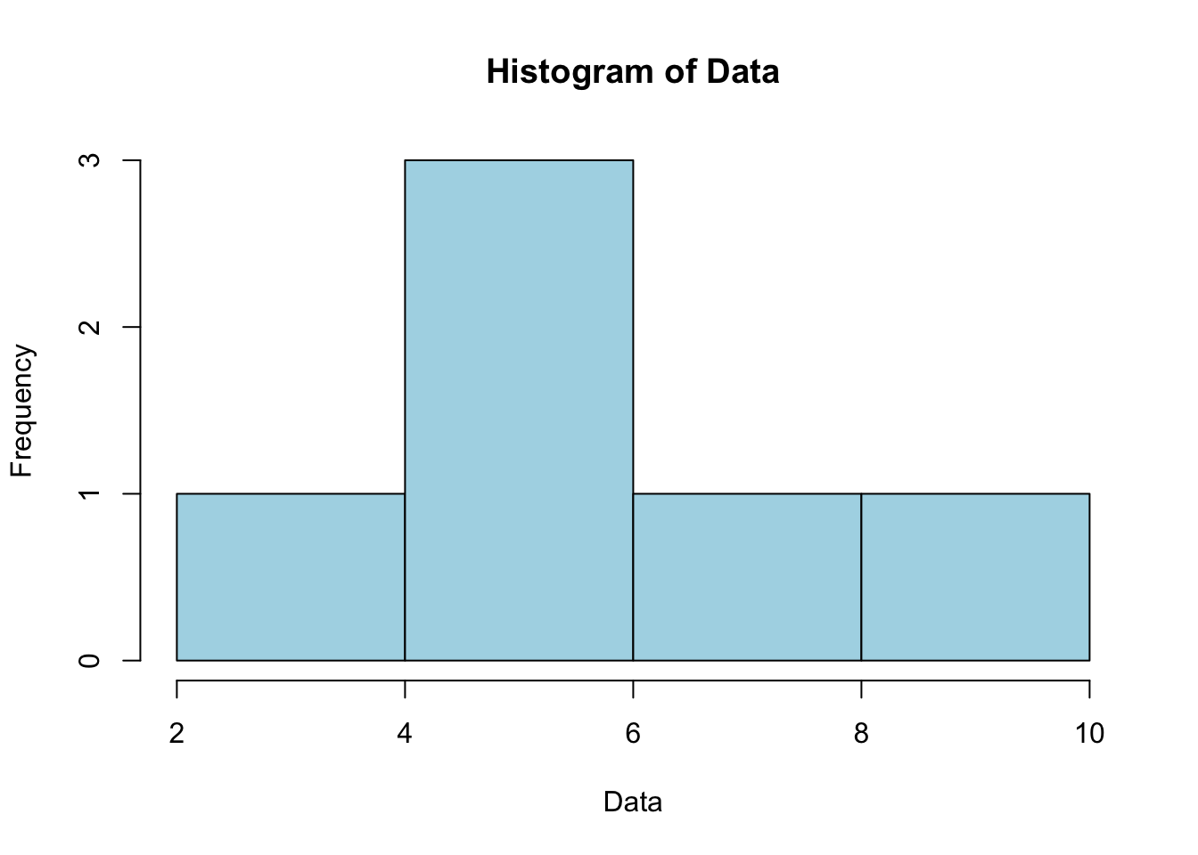
A boxplot provides a graphical representation of the minimum, first quartile, median, third quartile, and maximum. It also highlights outliers.
boxplot(data,
        main = "Boxplot of Data",
        ylab = "Values",
        col = "lightgreen")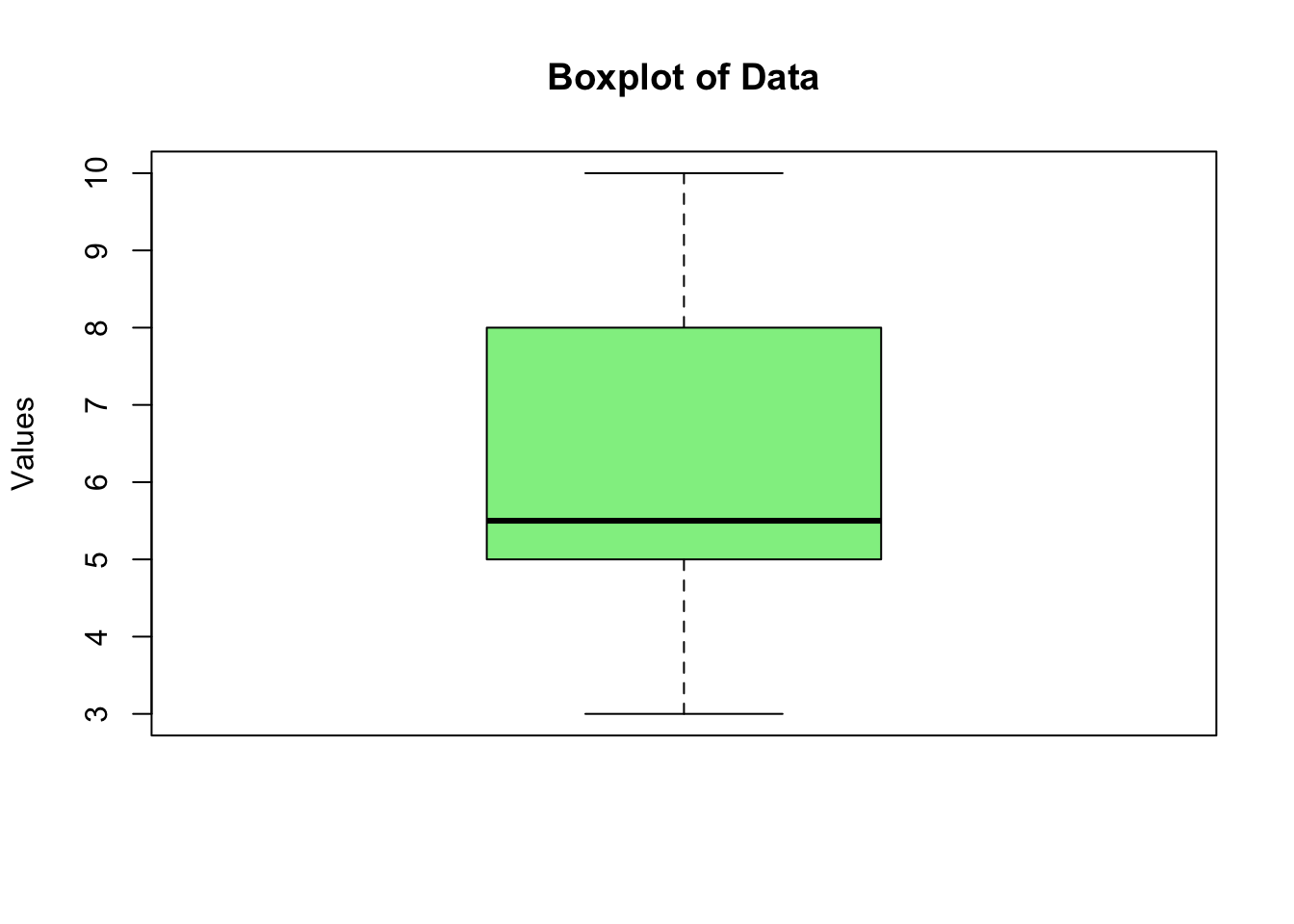
A density plot provides a smooth estimate of the distribution of the data, which can be useful to understand its overall shape.
plot(density(data),
     main = "Density Plot of Data",
     xlab = "Data",
     col = "blue")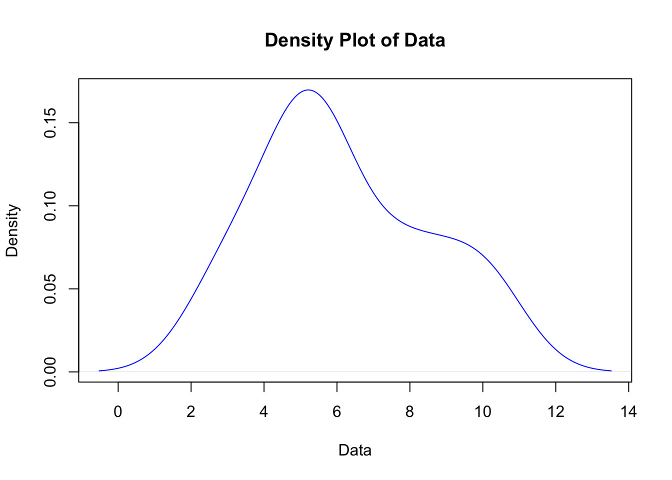
By using these visualizations, we can better understand the data distribution and assess properties such as skewness, kurtosis, and the presence of outliers.
1.2 Random Variables and Probability
In this section, we explore key concepts related to random variables and their probability distributions, as well as important theorems in probability theory.
A random variable is a numerical quantity whose value is determined by chance.
1.2.1 Probability Distributions
Here, we recall some of the most used probability distributions.
A probability distribution describes how the values of a random variable are distributed, describing the likelihood of different values occurring for a random variable. Below are some commonly used probability distributions.
The normal distribution, also known as the Gaussian distribution, is characterized by two parameters: the mean (\(\mu\)) and the standard deviation (\(\sigma\)). It is denoted as \(X \sim N(\mu, \sigma^2)\).
The probability density function (PDF) of a normal distribution is given by: \[ f(x) = \frac{1}{\sigma \sqrt{2\pi}} \exp\left(-\frac{(x - \mu)^2}{2\sigma^2}\right) \]
Parameters:
- \(\mu\): Mean of the distribution
- \(\sigma\): Standard deviation of the distribution
Characteristics:
- Bell-shaped curve
- Symmetric around the mean
- Mean, median, and mode are all equal to \(\mu\)
- Standard deviation parameter \(\sigma\) determines the spread of the distribution.
# Example of a normal distribution in R
x <- seq(-10, 10, length = 100)
mu <- 0  # mean
sigma <- 1  # standard deviation
# dnorm gives the density function
y <- dnorm(x, mean = mu, sd = sigma)

plot(x, y,
     type = "l",
     main = "Normal Distribution",
     xlab = "x",
     ylab = "Density")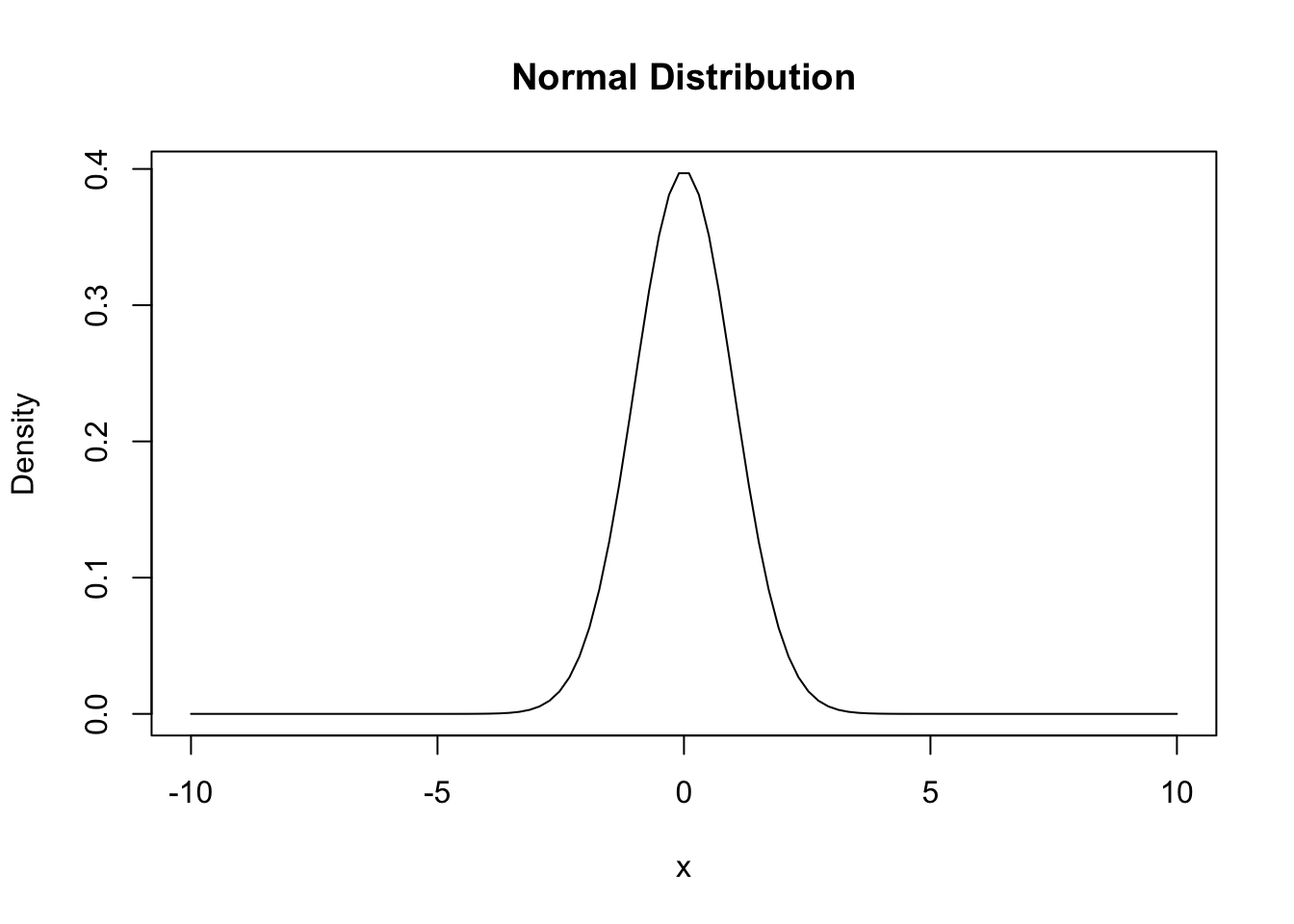
The binomial distribution describes the number of successes in a fixed number of independent Bernoulli trials, each with the same probability of success \(p\). It is denoted as \(X \sim B(n, p)\).
The probability mass function (PMF) is given by: \[ P(X = k) = \binom{n}{k} p^k (1 - p)^{n-k}, \quad k = 0, 1, 2, \dots, n \]
Parameters:
- \(n\): Number of trials
- \(p\): Probability of success in a single trial
Characteristics:
- Models the number of successes in a fixed number of independent Bernoulli trials
- Mean is \(np\)
- Variance is \(np(1−p)\)
n <- 10  # number of trials
p <- 0.5  # probability of success
x <- 0:n
y <- dbinom(x, size = n, prob = p)

barplot(y,
        names.arg = x,
        main = "Binomial Distribution",
        xlab = "Number of Successes",
        ylab = "Probability")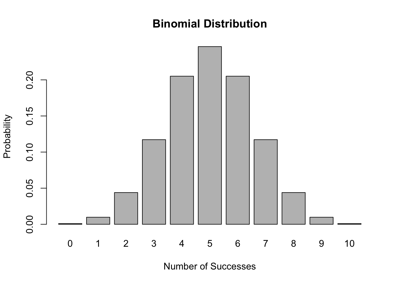
Student’s t-distribution is used when estimating the mean of a normally distributed population in situations where the sample size is small and population variance is unknown. It has a parameter, degrees of freedom (\(\nu\)), and is denoted as \(X \sim t_{\nu}\).
Fisher-Snedecor’s F-distribution is used to compare two variances by analyzing the ratio of two independent chi-squared variables. It has two parameters, the degrees of freedom of the numerator (\(d_1\)) and the degrees of freedom of the denominator (\(d_2\)), an is denoted as \(X \sim F(d_1, d_2)\).
Chi-Square distribution is used in tests of independence and goodness of fit. It is denoted as \(X \sim \chi^2_n\).
# Plotting t-distribution, F-distribution, and Chi-square distribution in R
# Student's t
x_t <- seq(-5, 5, length = 100)
y_t <- dt(x_t, df = 10)
# Ficher-Snedecor's F
x_f <- seq(0, 5, length = 100)
y_f <- df(x_f, df1 = 5, df2 = 2)
# Chi squared
x_chi <- seq(0, 10, length = 100)
y_chi <- dchisq(x_chi, df = 5)

# Plot t-distribution
plot(x_t, y_t,
     type = "l",
     main = "Student's t-Distribution",
     xlab = "x",
     ylab = "Density")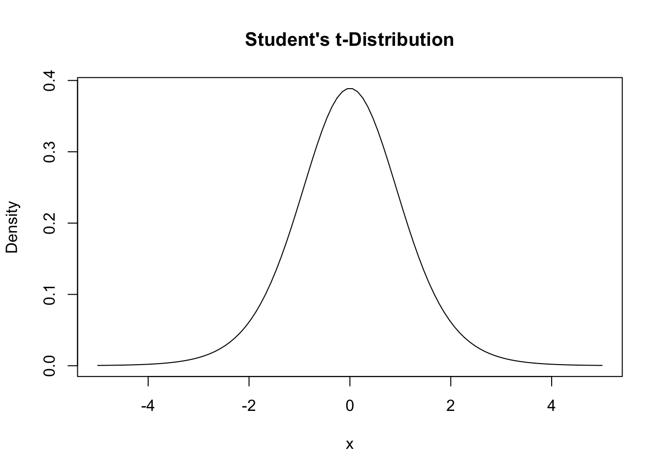
# Plot F-distribution
plot(x_f, y_f,
     type = "l",
     main = "F-Distribution",
     xlab = "x",
     ylab = "Density")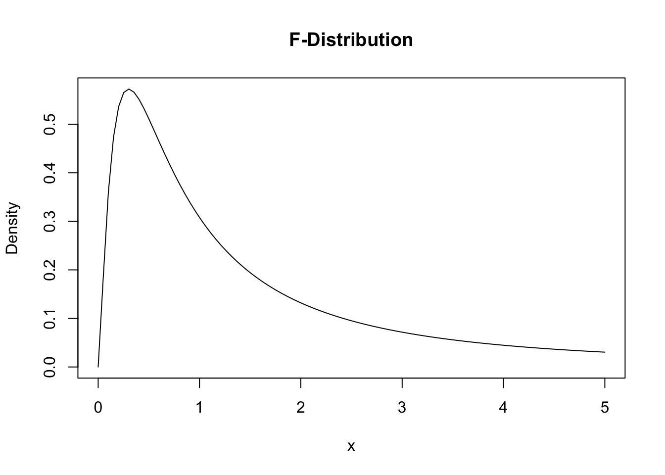
# Plot Chi-square distribution
plot(x_chi, y_chi,
     type = "l",
     main = "Chi-square Distribution",
     xlab = "x",
     ylab = "Density")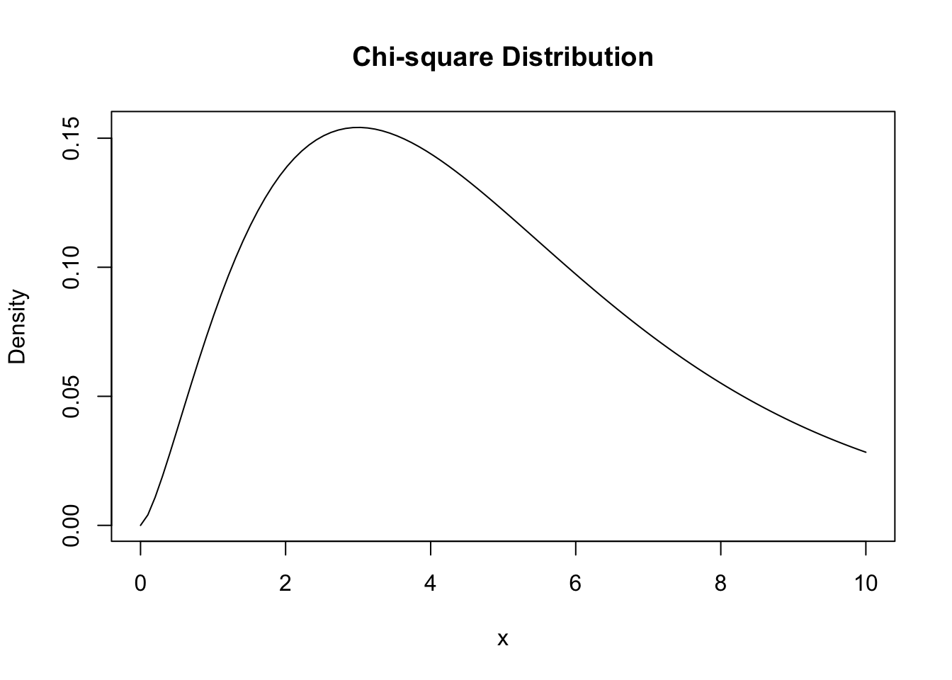
1.2.2 Probability Theory
The Total Probability Theorem is a fundamental rule that relates the probability of an event to the probabilities of conditional events that form a partition of the sample space.
If \(S_1, S_2, \dots, S_n\) is a partition of the sample space, then the total probability of event \(A\) is \[ P(A) = \sum_{i=1}^{n} P(A|S_i) P(S_i) \]
If \(S_1\) and \(S_2\) are two mutually exclusive events that form a partition of the sample space, then: \[ P(A) = P(A|S_1)P(S_1) + P(A|S_2)P(S_2) \]
Bayes’ theorem provides a way to update the probability of a hypothesis based on new evidence.
Given two events \(A\) and \(B\): \[ P(B|A) = \frac{P(B)P(A|B)}{P(A)} \] where:
- \(P(B|A)\) is the posterior probability: the probability of event \(B\) occurring given that \(A\) has occurred.
- \(P(A|B)\) is the likelihood: the probability of event \(A\) occurring given that \(B\) has occurred.
- \(P(B)\) is the prior probability: the initial estimate of the probability of \(B\).
- \(P(A)\) is the marginal likelihood: the total probability of \(A\).
prior_B <- 0.2  # P(B)
likelihood_A_given_B <- 0.8  # P(A|B)
prob_A <- 0.5  # P(A)

posterior_B_given_A <- (prior_B * likelihood_A_given_B) / prob_A
posterior_B_given_A  # P(B|A)
## [1] 0.32