3  Regression

3.1 Modelling techniques

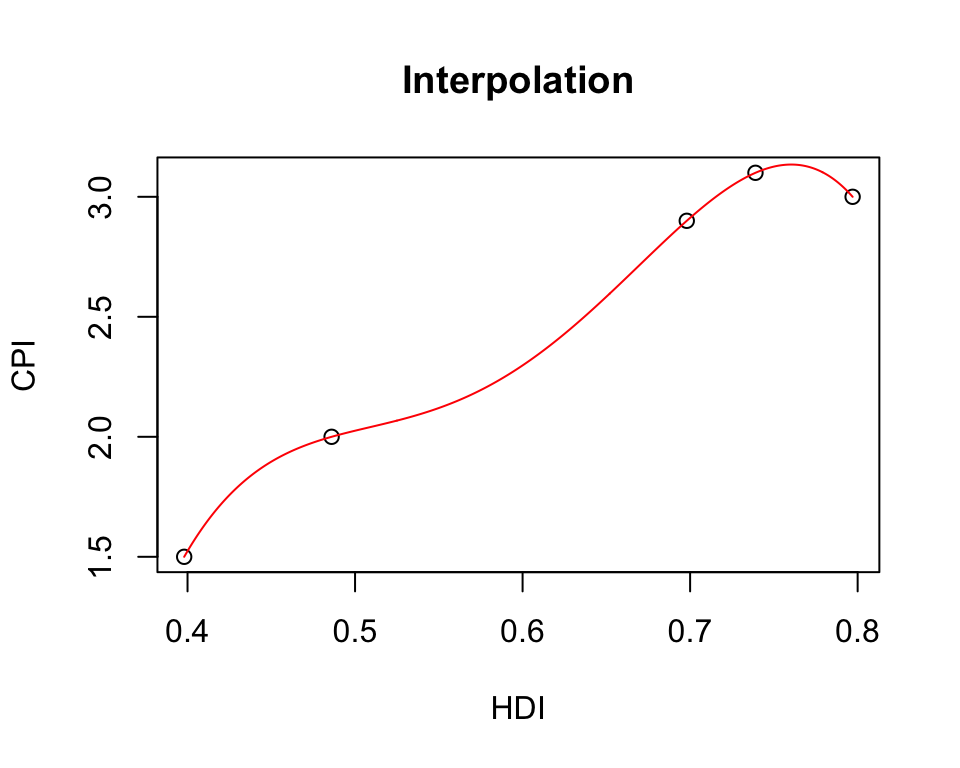
There are two types of basic numerical techniques to model the relationship between variables in a dataset: interpolation and approximation (adjustment).

In both cases, the goal is to get a function that best fits to a set of data (a cloud of data) from observations, data collected from sensors, datasets, etc.

Purpose:

• Prediction of future observations.
• Find relationships, functions between dataset variables.
• Description of the data structure.

3.1.1 Linear interpolation

The normal input is a data table \(\{(x_i,y_i)\}\) and the goal is to find an interpolating function \(\phi(x)=a_0+a_{1}f_{1}(x)\) (the easiest approach considers polynomial functions \(f_1(x)=x\)).

Then, the model will be: \[ \phi(x)=a_0+a_{1}x\] where:

• \(a_0\) is named the intercept.
• \(a_1\) is named the slope.

This tries to find a straight line that passes through all the data points. This will only happen if all \(\{(x_i, y_i)\}\) are collinear, which is not usually the case.

3.1.2 Polynomial interpolation

Assuming we have \(n+1\) points \(\{ (x_{0}, y_{0}), (x_{1}, y_{1}), (x_{2}, y_{2}), \ldots, (x_{n}, y_{n})\}\), polynomial interpolation consists of finding a polynomial function \(\phi(x)\) passing through the given points.

\[ \phi (x)=a_0+a_{1}x+a_{2}x^2+\ldots+a_{n}x^n\] Note that we are using that a basis of the polynomials of grade less than or equal to \(n\) is \(B=\{1, x,x^2,\ldots,x^n\}\).

If we impose \(y_i = \phi(x_i)\), we obtain the following equations: \[ \left. \begin{array}{lr} a_0+a_{1}x_{0}+a_{2}x_{0}^2+\ldots&=y_{0}\\ a_0+a_{1}x_{1}+a_{2}x_{1}^2+\ldots&=y_{1}\\ \ldots&\ldots\\ a_0+a_{1}x_{n}+a_{2}x_{n}^2+\ldots&=y_{n}\\ \\ \end{array}\right\}\]

This is a linear system that has a unique solution \(\vec{a} = (a_0, \ldots, a_n)\) if and only if all \(x_i\) are different.

3.1.3 Linear Regression: Minimizing the residual sum of squares

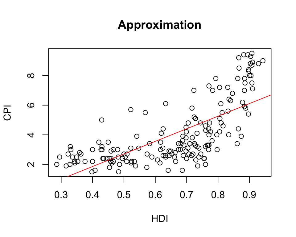
With a large number of observations, interpolation methods are not adequate, hence adjusting a linear regression model \(y=\phi(x) = a_0 + a_1x\) is used. Such a model reflects the effect of changing a variable \(x\) (independent variable) in variable \(y\) (dependent variable). It considers that there exist a linear relationship between the variables.

A common way to estimate the parameters of a statistical model is to adjust a function which minimize the errors. The most used method is that of minimizing the residual sum of squares, RSS, which is defined by: \[ RSS(\vec{a}):=\displaystyle\sum_{i=1}^{n}(y_i- (a_0 + a_1x_i))^2 \] where \(\vec{a} = (a_0, a_1)\).

To minimize the RSS, we just differentiate the above expression with respect to \(a_0\) and \(a_1\), equal to 0, and solve.

For those \(a_0, a_1\), we have the linear model that we want to explain the changes in variable \(y\) due to changes in variable \(x\).

Notes:

• Although regression is probably the most simple approach for supervised learning, linear regression is still a useful and widely used statistical learning method.
• Other more complex statistical learning approaches are generalizations of linear regression.

3.2 Linear regression with one predictor

The easier model is linear regression with one single predictor: \[ \phi(x) = a_0 + a_1 x\]

Finding this model is equivalent to finding a straight line that best fits the point cloud: \(y_i \approx \phi(x_i) = a_0 + a_1 x_i\), minimizing the RSS.

3.2.1 Linear regression using R

We use the lm() function.

regression.model <- lm(formula = y ~ x,  
                    data = dataset )  

• y is the dependent variable, the output.
• x is the independent variable, the predictor
• dataset a dataset with the attributes x and y.

If we want to apply lm() to the EconomistData dataset, we use the following:

# execute only the fist time
# install.packages("readr") 
require(readr)
library(readr)
CPIdata <- read_csv(
  here::here("data",
             "EconomistData.csv"))
attach(CPIdata)

# lm is a model formula
# ~ (read "is modeled as")
f1 <- lm(CPI ~ HDI)
f1
## 
## Call:
## lm(formula = CPI ~ HDI)
## 
## Coefficients:
## (Intercept)          HDI  
##      -1.540        8.497

# We can plot the model
plot(HDI, CPI)
abline(f1)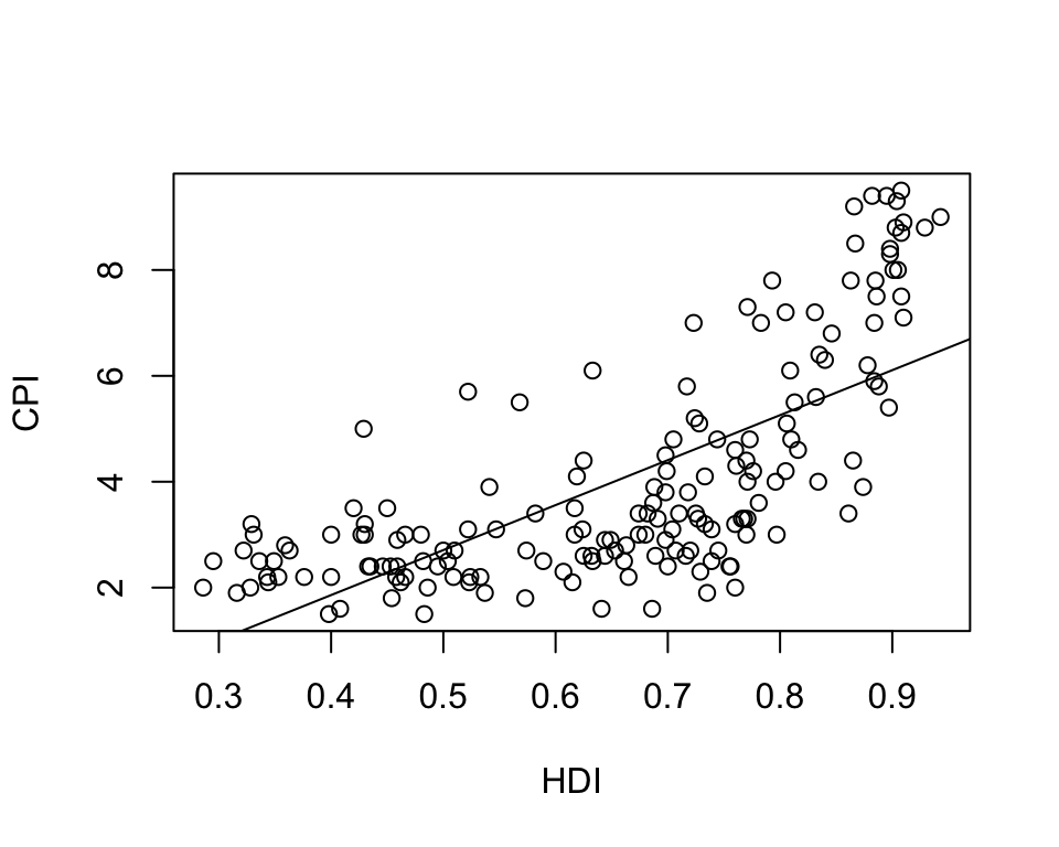  

The linear model is \[\phi(x)=-1.540 + 8.497x\]

Which is the meaning of the coefficient \(8.497\) (the slope)? If \(x\) is increased in 1, then \(Y\) is increased in 1

Which is the meaning of the coefficient \(-1.540\) (the intercept)? Value expected of \(y\), if \(x\) has a value of 0.

3.2.2 Goodness of fit

3.2.2.1 Residuals

If the points are not colinear, there will be a difference between \(y_i\) and the predicted value \(\overline{y} = \phi(x_i)\). This difference is called the residual \(\epsilon_i = y_i - \overline{y}\).

Thus, \(RSS(\vec{a}) = \| \epsilon \|_2^2= \displaystyle\sum_{i=1}^{N}{\epsilon_i}^2\)

We assume these residuals:

• They must have a zero average.
• If this is not the case, the bias must be measured.
• More points may need to be included in the data cloud.
• Errors must be uniformly distributed.
• We must wait for the residues to be uniformly distributed without patterns that detect anomalies.
  
• A first way would be to face the waste with the adjustment and the points should be around \(y=0\).

3.2.2.2 RSE

We define the Residual Standard Error as follows: \[RSE=\sqrt{\frac{1}{n-2} \,\, RSS}\]

RSE is an estimate of the standard deviation of \(\epsilon_i\).

RSE is considered a measure of the lack of fit of the model to the data.

• If the predictions using the model are very good, we can conclude that the model fits the data very well.

• On the other hand, if the model doesn’t fit the data well then the RSE may be quite large.

3.2.2.3 R-squared

R-squared (called the coefficient of determination) or fraction of variance explained is

\[R^2=1-\frac{RSS}{TSS}\] where \[TSS=\sum_{i=1}^n (y_i-\overline{y})\]

• RSE is an absolute measure of lack of fit of the model.

• \(R^2\) takes the form of a proportion measure (the proportion of variance explained), that is, the proportion of the variance in the outcome variable that can be accounted for by the predictor.

\(R^2\) can be estimated with the correlation \(r\) between the input (\(X\) variable) and the output (\(Y\) variable) as follows: \(R^2=r^2\).

If \(R^2\) is close to 1 indicates that a large proportion of the variability in the response has been explained by the regression. A number near 0 indicates that the linear model is wrong, or the inherent error is high, or both.

Note: The Pearson correlation is equivalent to running a linear regression model that uses only one predictor variable - the squared correlation \(r^2\) is identical to the \(R^2\) value for a linear regression with only a single predictor.

3.2.2.4 R-squared and Adjusted R-squared

R language returns Multiple R-squared and Adjusted R-squared.

If you add more predictors into the model, the \(R^2\) value will increase (or at least it will be the same). In a regression model with \(K\) predictors, fit to a data set containing \(N\) observations, the adjusted \(R^2\) is:

\[ \mbox{adj. } R^2 = 1 - \left(\frac{\mbox{SS}_{res}}{\mbox{SS}_{tot}} \times \frac{N-1}{N-K-1} \right) \]

The adjusted \(R^2\) value will only increase when the new variables improve the model performance.

3.2.3 Model quality with R

The main estimators can be found by executing the summary() function:

summary(f1)
## 
## Call:
## lm(formula = CPI ~ HDI)
## 
## Residuals:
##     Min      1Q  Median      3Q     Max 
## -2.9180 -1.1872 -0.2029  1.0744  3.4453 
## 
## Coefficients:
##             Estimate Std. Error t value Pr(>|t|)    
## (Intercept)  -1.5400     0.4453  -3.458 0.000686 ***
## HDI           8.4975     0.6539  12.994  < 2e-16 ***
## ---
## Signif. codes:  0 '***' 0.001 '**' 0.01 '*' 0.05 '.' 0.1 ' ' 1
## 
## Residual standard error: 1.506 on 171 degrees of freedom
## Multiple R-squared:  0.4968, Adjusted R-squared:  0.4939 
## F-statistic: 168.9 on 1 and 171 DF,  p-value: < 2.2e-16

From those results, we can explain the model quality objectively.

We can also use plots to graph certain relationships between the residuals and the fitted values (\(\phi(x_i)\)) and check whether the residuals have 0 average, for instance.

We can check if the fitted curve (with the predicted values) fits the data cloud:

plot(HDI, CPI, col = "red")
par(new = TRUE)
plot(HDI,
     predict(f1, 
             data.frame(x = HDI)),
     ylab = "Predicted")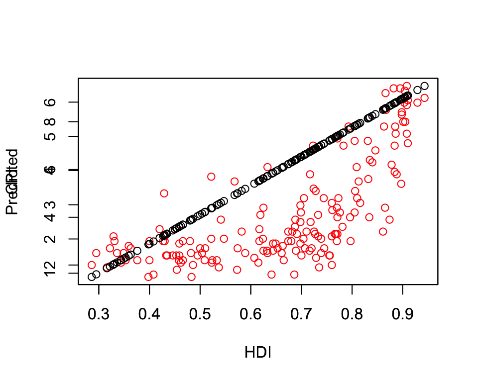

We get the fitted values with the fitted() function and the residuals with residuals() (easy to remember, aren’t they?)

# Fitted values
head(fitted(f1))
##        1        2        3        4        5        6 
## 1.841949 4.739580 4.391184 2.589725 5.232432 4.544139
# Residuals
head(residuals(f1))
##          1          2          3          4          5          6 
## -0.3419488 -1.6395800 -1.4911844 -0.5897246 -2.2324322 -1.9441386

We can check the distribution of the residuals by using histograms or density plots:

hist(residuals(f1))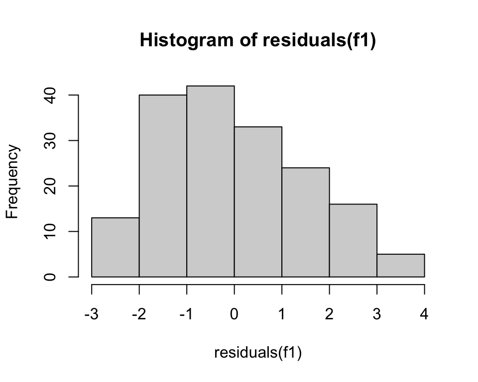

plot(density(residuals(f1)))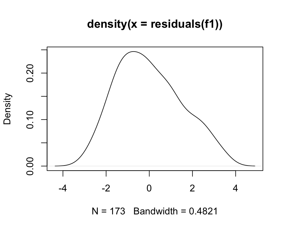

• Import ToyotaCorolla dataset from the course website.
• Build linear models m1, m2 using Multiple Linear Regression.
• Analyze the goodness of fit and model quality, explaining the results.

3.2.4 Are the coefficients meaningful?

We have obtained some coefficients:

coef(f1)
## (Intercept)         HDI 
##   -1.540037    8.497452

but we do not know if these coefficients are indeed significant in the model or not.

To test whether they are meaningful in the model, it is used a statistical test.

This will explained later in the multiple linear regression.

3.2.5 How to generalize this linear regression

The linear model \(\phi(x) = a_0 + a_1 x\) could be generalized in several ways.

We can also apply linear regression to more than 1 variable \(x=\{x_1, x_2\}\).

For example, consider modeling temperature as a function of location \(\{x_1,x_2\}\).

\[ \phi(x) = a_0 + a_1 x_1 + a_2x_2\] or even, \[ \phi_2(x) =a_0 + a_1x_1 + a_2x_2 + a_3x_1^2\]

Note: it is possible to model non-linear relationships. In general, a simple approach (we could use non-polynomial functions) is considered using polynomial basis functions, where the model has the form

\[\phi(x)=a_0+a_1x+a_2x^2+ \ldots+ a_nx^n\]

3.3 Multiple Linear Regression

Given a set of variables \(X_1, X_2, \dots, X_m\), multiple linear regression computes the next model:

\[\phi(\vec{X})=a_0+a_1X_1+a_2X_2+\dots, a_mX_m+\epsilon=Y\] In this model a coefficient \(a_j\) is interpreted as the average effect on \(Y\) of a one unit increase in \(X_j\), holding all other predictors fixed.

The ideal scenario is when the predictors are uncorrelated and in this case each coefficient can be estimated and tested separately.

Correlations amongst predictors cause problems because the variance of all coefficients tends to increase, sometimes dramatically.

Normally the independence is a utopia. Normally, predictors usually change together.

NOTE EVERYTHING that we have already explained for the case with one predictor is also valid for the remaining of this explanation: RSE, residuals, plots, etc.

3.3.1 Adding predictors with R

The formula in the lm() can be extended with more predictor variables in the right-hand side:

modelo1 <- lm(HDI.Rank ~ CPI + HDI)

3.3.2 Evaluating the Regression Coefficients

\[\phi(x)=a_0+a_1X_1+a_2X_2+\dots, a_mX_m\]

3.3.2.1 F-statistic

We establish the null hypothesis:

\[H_O: a_0 = a_1 = a_2= \dots= a_m= 0\] Null hypothesis: there is no relationship between the predictors and the outcome

versus the alternative \[H_a: \mbox{ at least one } a_i \mbox{ is non-zero}\] Alternative hypothesis: the data are distributed as the regression model predicts

The hypothesis test is performed by means of F-statistic:

\[F=\frac{(TSS-RSS)/p}{RSS/(n-m-1)}\]

where

\[TSS = \sum (y_i − \overline{y} )^2\]

When there is no relationship between the real valor and predictors, the F-statistic must take a value close to 1.

• If \(H_a\) is true the F-value must be greater than 1.

• If F-value is closer to 1, the answer to reject the hypothesis depends on values of \(n\) and \(m\).

• Using the F-value, the p-value is computed.

3.3.2.2 p-value

Using p-value we can determine whether or not to reject \(H_0\).

3.3.2.3 Evaluating the coefficients in R

summary(modelo1)
## 
## Call:
## lm(formula = HDI.Rank ~ CPI + HDI)
## 
## Residuals:
##      Min       1Q   Median       3Q      Max 
## -19.9326  -6.5788  -0.5189   5.9769  21.6061 
## 
## Coefficients:
##              Estimate Std. Error t value Pr(>|t|)    
## (Intercept)  293.9914     2.5014 117.529  < 2e-16 ***
## CPI           -2.9350     0.4153  -7.068 3.89e-11 ***
## HDI         -283.8765     5.0064 -56.703  < 2e-16 ***
## ---
## Signif. codes:  0 '***' 0.001 '**' 0.01 '*' 0.05 '.' 0.1 ' ' 1
## 
## Residual standard error: 8.178 on 170 degrees of freedom
## Multiple R-squared:  0.9782, Adjusted R-squared:  0.9779 
## F-statistic:  3806 on 2 and 170 DF,  p-value: < 2.2e-16

• p-value is essentially 0: extremely strong evidence that at least one of the media is associated with output variable.
• R returns the \(p\)-value for each coefficient: These provide information about whether each individual predictor is related to the response, after adjusting for the other predictors.
• If, for a given coefficient, \(Pr(>|t|) \approx 0\), the coefficient is significant - see *** in each row of the table.
• F-value is 3806 (must be greater than 1).
  
• \(p\)-value is close to 0.
• degrees of freedom: The number of independent pieces of information used in the estimation of a parameter.
• Multiple R-squared is used for evaluating how well your model fits the data. 97% of the variability in HDI.Rank is explained by CPI+HDI.
• (Multiple R squared) measures the amount of variation in the response variable that can be explained by the predictor variables.
• Adjusted Rsquared adds penalties for the number of predictors in the model. Therefore it shows a balance between the most parsimonious model, and the best fitting model ( ratio between the number of observations and the predictors). If you have a large difference between your multiple and your adjusted Rsquared that indicates you may have overfit your model.

3.3.3 Improving the models

Trying a more complicated model

• Polynomial regression.
• Polynomial orthogonal regression.
• Non linear regression.
• etc.

3.3.3.1 Classical polynomial approach

Trying a polynomial of degree \(n\) for \(\phi(x)\).

We add to the model the term I(X_i^n).

poli.2c <- lm(CPI ~ HDI + I(HDI^2))
poli.3c <- lm(CPI ~ HDI + I(HDI^2) + I(HDI^3))
poli.4c <- lm(CPI ~ HDI + I(HDI^2) + I(HDI^3)+ I(HDI^4))
poli.2c
## 
## Call:
## lm(formula = CPI ~ HDI + I(HDI^2))
## 
## Coefficients:
## (Intercept)          HDI     I(HDI^2)  
##       9.552      -30.051       30.785
poli.3c
## 
## Call:
## lm(formula = CPI ~ HDI + I(HDI^2) + I(HDI^3))
## 
## Coefficients:
## (Intercept)          HDI     I(HDI^2)     I(HDI^3)  
##      -7.116       59.605     -119.817       80.060
poli.4c
## 
## Call:
## lm(formula = CPI ~ HDI + I(HDI^2) + I(HDI^3) + I(HDI^4))
## 
## Coefficients:
## (Intercept)          HDI     I(HDI^2)     I(HDI^3)     I(HDI^4)  
##    -0.08463      7.38593     18.62201    -75.89626     63.32330

We can check the goodness of fit for any of these models:

plot(HDI, CPI, col = "red", ylab = "")
par(new = TRUE)
plot(HDI,
     predict(poli.2c, 
             data.frame(x = HDI)),
     ylab = "Predicted")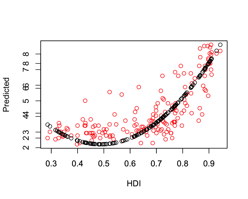

3.3.3.2 Orthogonal polynomial approach

We will use poly(X_i, n) to consider a new orthogonal polynomial of degree n.

poli.2o <- lm(CPI ~ poly(HDI, 2))
poli.3o <- lm(CPI ~ poly(HDI, 3))
poli.4o <- lm(CPI ~ poly(HDI, 4))
poli.2o
## 
## Call:
## lm(formula = CPI ~ poly(HDI, 2))
## 
## Coefficients:
##   (Intercept)  poly(HDI, 2)1  poly(HDI, 2)2  
##         4.052         19.568         11.859
poli.3o
## 
## Call:
## lm(formula = CPI ~ poly(HDI, 3))
## 
## Coefficients:
##   (Intercept)  poly(HDI, 3)1  poly(HDI, 3)2  poly(HDI, 3)3  
##         4.052         19.568         11.859          5.159
poli.4o
## 
## Call:
## lm(formula = CPI ~ poly(HDI, 4))
## 
## Coefficients:
##   (Intercept)  poly(HDI, 4)1  poly(HDI, 4)2  poly(HDI, 4)3  poly(HDI, 4)4  
##        4.0520        19.5681        11.8590         5.1587         0.6239

3.3.3.3 Updating a pre-existing model

To update a model and add new predictors, we use the update() function.

p1 <- lm(CPI ~ HDI)
p2 <- update(p1, . ~ . + I(HDI^2))
p3 <- update(p2, . ~ . + I(HDI^3))
p4 <- update(p3, . ~ . + I(HDI^4))
p5 <- update(p4, . ~ . + I(HDI^5))
p6 <- update(p5, . ~ . + I(HDI^6))
p7 <- update(p6, . ~ . + I(HDI^7))

Exercise

• With the ToyotaCorolla dataset, build two polynomial and orthogonal models, and call them m3 and m4.
• Repeat the analysis made for m1 and m2. Also, analyze the significancy of the regression coefficients.

3.3.4 Comparing models with ANOVA

ANOVA (ANalysis Of VAriance) performs the Chi-square test to compare the models obtaining if the reduction in the residual sum of squares are statistically significant or not.

f1
## 
## Call:
## lm(formula = CPI ~ HDI)
## 
## Coefficients:
## (Intercept)          HDI  
##      -1.540        8.497
poli.2c
## 
## Call:
## lm(formula = CPI ~ HDI + I(HDI^2))
## 
## Coefficients:
## (Intercept)          HDI     I(HDI^2)  
##       9.552      -30.051       30.785
anova(f1, poli.2c) # We can add more models
## Analysis of Variance Table
## 
## Model 1: CPI ~ HDI
## Model 2: CPI ~ HDI + I(HDI^2)
##   Res.Df    RSS Df Sum of Sq      F    Pr(>F)    
## 1    171 387.78                                  
## 2    170 247.14  1    140.63 96.737 < 2.2e-16 ***
## ---
## Signif. codes:  0 '***' 0.001 '**' 0.01 '*' 0.05 '.' 0.1 ' ' 1

The parameter \(Pr (>F)\) is the probability that rejecting null hypothesis (the most complex model does not fit better than the simplest model) could be an error.

• Note: the second model must be an extended model of the first model.

Exercise

Compare all the models built for ToyotaCorolla using ANOVA and explain the results.

3.3.5 Interactions

Given a set of variables \(A, B, X, Y, Z, U\) we can test the following models, in addition to the combinations of these with the linear and polynomial models previously seen.

• \(+\): combinations (\(A+B\))
• \(:\): interactions (\(A:B\)). Meaning of interactions
• \(*\) combinations and interactions (\(A*B = A+B+A:B\))
• \(.\) (combinations of all variables )

Examples:

# f1(X)=aY + bZ 
f1 <- lm( X ~ Y + Z )

# f2(X)=a(Y+Z) + bU 
f2 <- lm( X ~ I(Y + Z) + U )

#f3(X)=aY + bY^2+cZ
f3 <- lm( X ~ I(Y) + I(Y^2) + I(Z) )
f3 <- lm( X ~   Y + I(Y^2) +     Z )

# f4(X): interactions 
f4 <- lm( X ~ Y:Z )

# f5(X): interactions with the rest of variables
f5 <- lm( X ~ . )

3.4 Regression in R - Analysing Boston dataset

This dataset stores the Housing Values in Suburbs of Boston.

# package with a lot of datasets
library (MASS) # install if error
data(Boston) #Housing Values in Suburbs of Boston
names(Boston)
# ?Boston # See the descriptions of columns

3.4.1 Fit a simple linear regression

\[medv=\phi(lstat)=a_0+a_1\, lstat\]

• lstat: lower status of the population (percent).
• medv: median value of owner-occupied homes in $1000s.

lm.fit <- lm(medv ~ lstat,
             data = Boston)
lm.fit

The model found is: \[medv=\phi(lstat)=34.55-0.95\, lstat\]

3.4.2 Analyzing the model

For more detailed information:

summary(lm.fit)

For more information we can use names with the linear model:

names(lm.fit)
# we ask for these information
coefficients(lm.fit)

Confidence interval for the coefficient estimates:

confint(lm.fit)

Visualizing the dataset+model:

attach(Boston)
# differents plots
plot(lstat, medv, col = "red ")
plot(lstat, medv, pch = 20)
plot(lstat, medv, pch = "+")
abline(lm.fit)
abline(lm.fit, lwd = 3)
abline(lm.fit, lwd = 3, col = "red")

3.4.3 Visualizing the linear model

oldpar <- par(mfrow = c(2, 2))
# divides the plotting region into a 2 × 2 grid of panels
plot(lm.fit)
par(oldpar)

3.4.4 Regression Diagnostics

• residuals
• rstudent
• cooks.distance

Search for information of these estimators, use with the dataset and explain.

Some plots regarding residuals, etc…

plot(predict(lm.fit), 
     residuals(lm.fit))
plot(predict(lm.fit), 
     rstudent(lm.fit))

• hatvalues(): On the basis of the residual plots, there is some evidence of non-linearity. Leverage statistics can be computed for any number of predictors using this function.

plot(hatvalues(lm.fit ))
which.max(hatvalues(lm.fit))

• which.max(): function identifies the index of the largest element of a vector. In this case, it tells us which observation has the largest leverage statistic.

3.4.5 Multiple regression

Fitting a model trying the regression with two input variables.

• lstat: lower status of the population (percent).
• medv: median value of owner-occupied homes in $1000s.
• age: age proportion of owner-occupied units built prior to 1940.

\[medv=\phi(lstat,age)=a_0+a_1\, lstat+ +a_2\, age\]

lm.fit2 <- lm(medv~lstat+age, data = Boston)
lm.fit2
summary(lm.fit2)

Data set contains 13 variables, how to select the best variables?:

• Facing the output variable against the rest of variables
• Analyzing the summary of the model.

lm.fit3 <- lm(medv ~ ., 
              data = Boston)
summary(lm.fit3)

3.4.5.1 Interaction terms

lm.fit4 <- lm(medv ~ lstat * age,
              data = Boston)
summary(lm.fit4)

3.4.5.2 Non-linear transformations of the predictors

lm.fit5 <- lm(medv ~ lstat + I(lstat^2),
              data = Boston)
summary(lm.fit5)

The \(p\)-value associated with the quadratic term suggests that lm.fit5 is an improved model.

3.4.5.3 Using ANOVA

Fist, we compare the model: linear (lm.fit) and quadratic (lm.fit5). If we represent these models, we could extract some important ideas:

#par(mfrow=c(2,2))
plot(lm.fit)
#par(mfrow=c(2,2))
plot(lm.fit5)

We can see a non-linearity in the relationship between medv and lstat.

Now, we will use anova() to perform a hypothesis test comparing the models.

anova(lm.fit, lm.fit5)

Interpretation: The null hypothesis says that the two models fit the data equally well, and the alternative hypothesis is that the extended model is superior.

See the F-statistic and the p-value associated.

This provides very clear evidence that the model containing the predictors \(lstat\) and \(lstat^2\) is better than the model with just the predictor \(lstat\).

3.5 Logistic Regression

3.5.1 Introduction

Logistic regression is an excellent tool for predicting the likelihood of something happening or not. It is used for classification tasks in quantitatives and qualitatives domains.

Firstly, we remind that linear regression corresponds to the family

\[p(y\mid x ;\theta)=\cal{N}(y;\theta^{\top} x;I)\]

To be used in the classification scenario it is necessary to define a different family of probability distributions. If we have two classes, class 0 and class 1, then we need only specify the probability of one of these classes.

The normal distribution over real-valued numbers that we used for linear regression is parametrized in terms of a mean. Any value we supply for this mean is valid. A distribution over a binary variable is slightly more complicated, because its mean must always be between 0 and 1.

For this task, logistic regression builds a linear model based on a transformed target variable.

As a summary, in Logistic Regression the output variable \(Y\) is binary, the input variables can be quantitative or qualitative and the distribution used is a binomial.

3.5.2 Binary response

As we have said, in linear regression we have:

\[y=f(X)=f(x_1,x_2,\ldots,x_k)=a_o+a_1x_1+\ldots+a_k x_k+\epsilon\]

The error \(\epsilon\) follows a normal distribution with mean zero.

In logistic regression the response variable can be either true (success) or false (failure).

For a binary response, the conditional mean in the regression model becomes \(P(y=1\mid X)\).

An acceptable function must always have values between 0 and 1. We want a response model where \(p\) is between 0 and 1.

\[p(X)=P(y=1\mid X)=f(a_o+a_1x_1+\ldots+a_k x_k)\]

The logistic regression model links the predictor variables to probabilities through the equation

\[p=P(y=1\mid X)=f(a_o+a_1x_1+\ldots+a_k x_k)=\displaystyle\frac{e^{a_o+a_1x_1+\ldots+a_k x_k}}{1+e^{a_o+a_1x_1+\ldots+a_k x_k}}\]

This function leads to S-shaped curves between 0 and 1 such as those shown in the next graph.

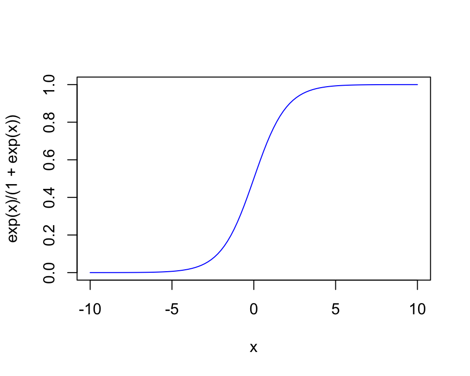
Using algebra we have:

\[\log\frac{p}{1-p}=a_o+a_1x_1+\ldots+a_k x_k\]

The quantity \(\frac{p}{(1 − p)}\) relates the probability of success, \(p\), to the probability of failure \((1 − p)\).

• We refer to \(\frac{p}{(1 − p)}\) as the odds of success.
• The quantity \(\log\frac{p}{1-p}\) is referred to as the logit of \(p\) and expresses the log odds of success.

Logistic regression, with its logit link \(\log\frac{p}{1-p}\) modeled as a linear function of the predictor variables, is the most popular model for a binary outcome variable.

3.5.3 Logistic regression in R

• The R command glm() is used to fit logistic regression models.
• glm() is a very general routine (used for other kinds of regressions).

It can be used to fit generalized linear models (hence its name):

• listing the linear predictors,
• defining the error distribution,
• specifying a link function.

For logistic regression, the family of the error distribution is the binomial. The default, family = binomial [or family = binomial(link = "logit")] specifies the logistic regression model.

f_1 <- glm(formula, family = binomial, data)

Remember that \[\mbox{if } f_1(X)=a_0+a_1x_1+a_2x_2\ldots \mbox{ then } p=\frac{\mathrm{e}^{f_1(X)}}{1+\mathrm{e}^{f_1(X)}}\]

3.5.4 Example

(From Logistic regression with glm)

We’ll use the diamonds dataset:

# First time install
# install.package(yarr)
library(yarrr)
head(diamonds)
##   weight clarity color value
## 1   9.35    0.88     4 182.5
## 2  11.10    1.05     5 191.2
## 3   8.65    0.85     6 175.7
## 4  10.43    1.15     5 195.2
## 5  10.62    0.92     5 181.6
## 6  12.35    0.44     4 182.9

Steps:

• Create a binary variable called value.g190 indicating whether the value of a diamond is greater than 190 or not.

diamonds$value.g190 <- diamonds$value > 190

• Use logistic regression with this new variable as output.

g.mod1 <- glm(formula = value.g190 ~ weight  + clarity + color, 
              data = diamonds, 
              family = binomial)
g.mod1
## 
## Call:  glm(formula = value.g190 ~ weight + clarity + color, family = binomial, 
##     data = diamonds)
## 
## Coefficients:
## (Intercept)       weight      clarity        color  
##    -18.8009       1.1251       9.2910      -0.3836  
## 
## Degrees of Freedom: 149 Total (i.e. Null);  146 Residual
## Null Deviance:       207.5 
## Residual Deviance: 106.7     AIC: 114.7
summary(g.mod1)
## 
## Call:
## glm(formula = value.g190 ~ weight + clarity + color, family = binomial, 
##     data = diamonds)
## 
## Coefficients:
##             Estimate Std. Error z value Pr(>|z|)    
## (Intercept) -18.8009     3.4634  -5.428 5.69e-08 ***
## weight        1.1251     0.1968   5.716 1.09e-08 ***
## clarity       9.2910     1.9629   4.733 2.21e-06 ***
## color        -0.3836     0.2481  -1.547    0.122    
## ---
## Signif. codes:  0 '***' 0.001 '**' 0.01 '*' 0.05 '.' 0.1 ' ' 1
## 
## (Dispersion parameter for binomial family taken to be 1)
## 
##     Null deviance: 207.52  on 149  degrees of freedom
## Residual deviance: 106.67  on 146  degrees of freedom
## AIC: 114.67
## 
## Number of Fisher Scoring iterations: 6

\[V(x) = -18.8009 + 1.1251 \mbox{ weight }+ 9.2910 \mbox{ clarity} -0.3836 \mbox{ color}\]

• Are all the variables significant?

diamonds$fitted.value <- g.mod1$fitted.values
head(diamonds[c("weight", "clarity", "color", "value", "fitted.value")])
##   weight clarity color value fitted.value
## 1   9.35    0.88     4 182.5   0.16251772
## 2  11.10    1.05     5 191.2   0.82129665
## 3   8.65    0.85     6 175.7   0.03008442
## 4  10.43    1.15     5 195.2   0.84559083
## 5  10.62    0.92     5 181.6   0.44454833
## 6  12.35    0.44     4 182.9   0.08688269

To use this regression with a new diamond:

# We build a new data frame
# It may have more than 1 row
d.new <- data.frame(weight = 12, 
                    clarity = 1.3,
                    color = 5)
# Evaluating in the model
# We obtain a prediction for each 
# row of the "newdata" data frame
logit <- predict(g.mod1, 
                 newdata = d.new)

This value is the logit-transformed probabilities. To compute the actual probability:

\[p=\frac{\mathrm{e}^{V(x)}}{1+\mathrm{e}^{V(x)}}=\frac{1}{1+\mathrm{e}^{-V(x)}}\]

p <- 1 / (1 + exp(-logit))
p
##         1 
## 0.9923129

This means that the new diamond will be valued over 190 with a probability of 99.23%.