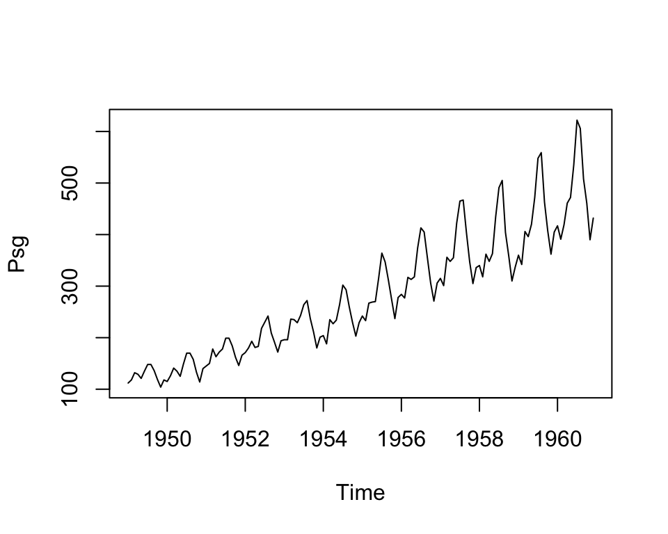
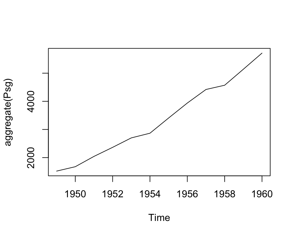
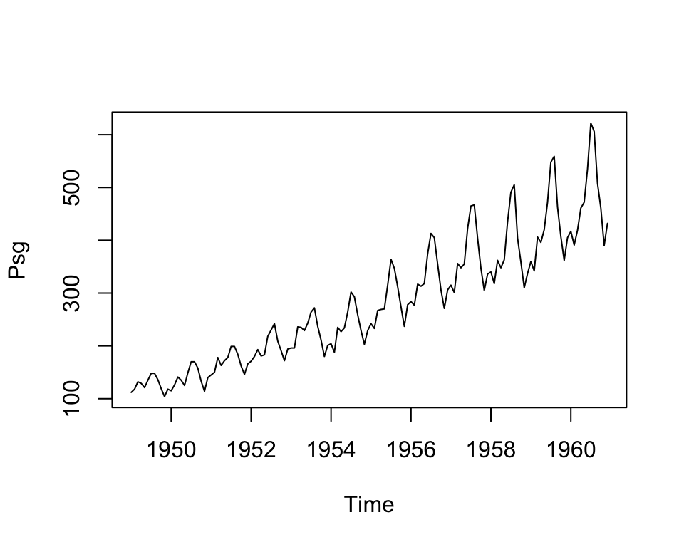
Singapore Airlines placed an initial order for twenty Boeing 787-9s and signed an order of intent to buy twenty-nine new Airbus planes, twenty A350s, and nine A380s (superjumbos). The airline’s decision to expand its fleet relied on a combination of time series analysis of airline passenger trends and corporate plans for maintaining or increasing its market share.
Gas suppliers - Variation about the average for the time of year depends on temperature and, to some extent, the wind speed. Time series analysis is used to forecast demand from the seasonal average with adjustments based on one-day-ahead weather forecasts.
Tell us what the future holds, so we may know that you are gods. (Isaiah 41:23)
Forecasting is the set of techniques modelling how to predict the future as accurately as possible, given all of the information available, including historical data and any future data. These methods try to extrapolate trend and seasonal patterns
Applications of Forecasting
Medicine, epidemiology,
planning for the economy features of a country, financial institutions, pocily organizations,
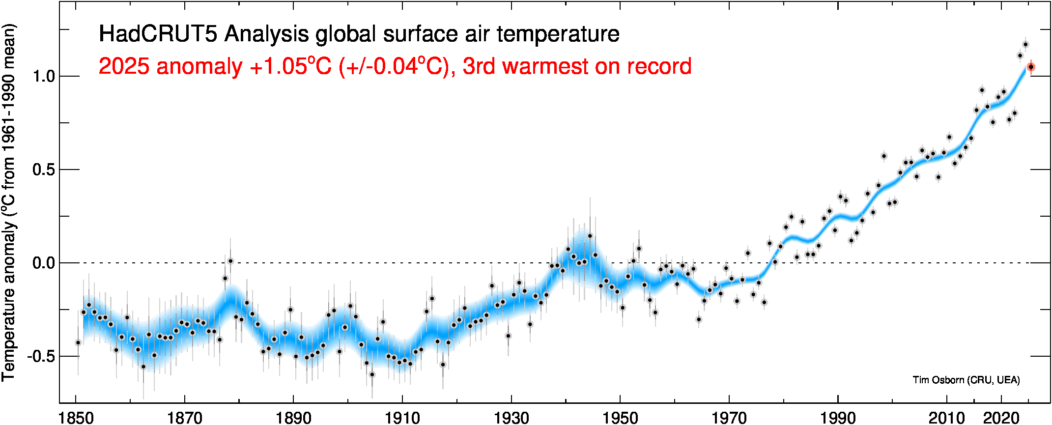
weather, global temperature changes
scheduling in bussiness,
marketing,
predicting sales in a shop,
finance and risk management,
prediction of population in a country, in a region,
seismic recordings
planning th stock of product in a online shop,
deciding whether to build another power generation plant,
scheduling personal in a call centre depending of the number of calls,
The study of adjacent points using conventional statistical methods have problems.
Conventional statistical methods are dependent on the assumption that these adjacent observations are independent and identically distributed.
The temporal data appears temporal correlations and ad-hoc techniques have been developed to treat these data.
Basic steps
Problem study
Data collection
Data analysis
Model selection and fitting
Model validation
Forecasting model deployment
Monitoring forecasting model performance
5.2.1 Time Series in R
5.2.1.1 Importing time series
To analyse your time series data we need to read it into R, and to plot the time series.
You can read data into R using scan(), which assumes that your data for successive time points is in a simple text file with one column.
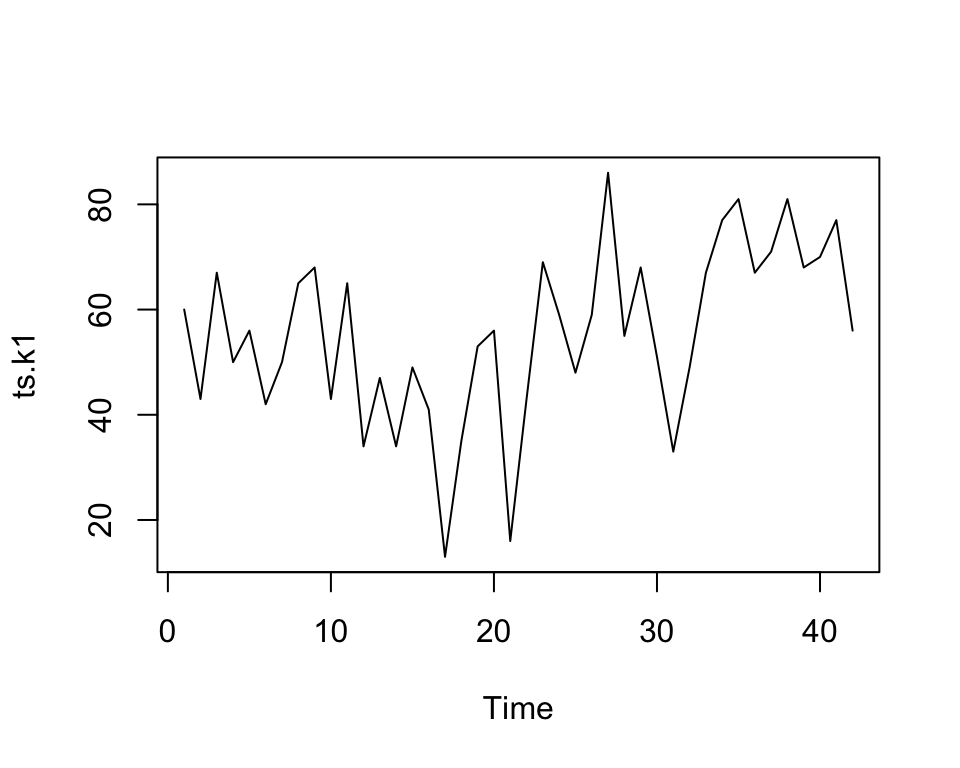
The file ts_k1.dat contains data about average business sales of a product.
# Read from an URL# Skip 1 line - commentdata.ts.k1 <-scan( here::here("data","ts_k1.dat"), skip =1)head(data.ts.k1)## [1] 60 43 67 50 56 42
The next step is to store the data in a time series object in R.
A time series is a list of numbers with temporal information stored as a ts object in R
There is a lot of packages and functions to deal with time series. Firstly, we will use ts function, which is used to create time-series objects.
The sintax of ts function is:
serie_1<-ts(data, start, end, frequency)# data - the values in the time series# start - the first forecast observations in a time series# end - the last observation in a time series# frequency - periods (month, quarter, annual)# frequency=1 (by default) - no periods or season in your data# frequency=12 - period is monthly# frequency=4 - period is quarterly#Example# data <- c(2, 8, 6, 10,# 5, 14, 7, 14,# 9, 23, 11, 29, 12)# serie1 <- ts(data,start = c(2023,1),frequency = 12)# plot(serie1)# autoplot(serie1) - ggplot of the ts object
If the data set has values for periods less than one year, for example, monthly or quarterly, one can specify the number of times that data was collected per year by using the ‘frequency’ parameter in the ts function.
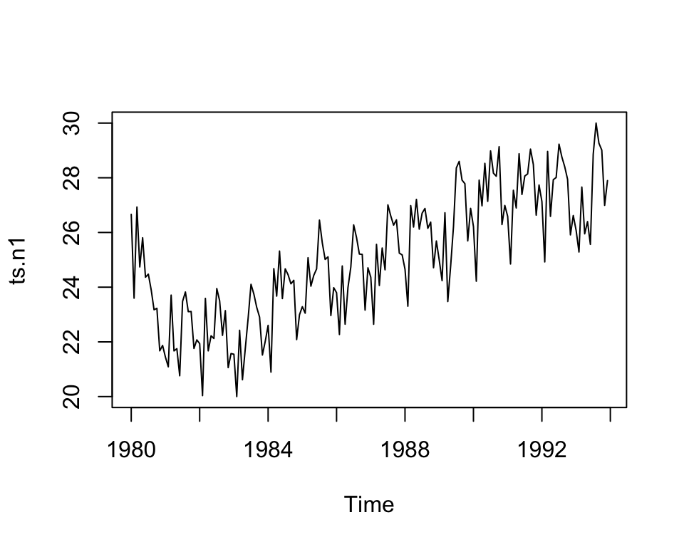
Let us make a basic plot of the time series data (for the two first datasets):
plot.ts(ts.k1)
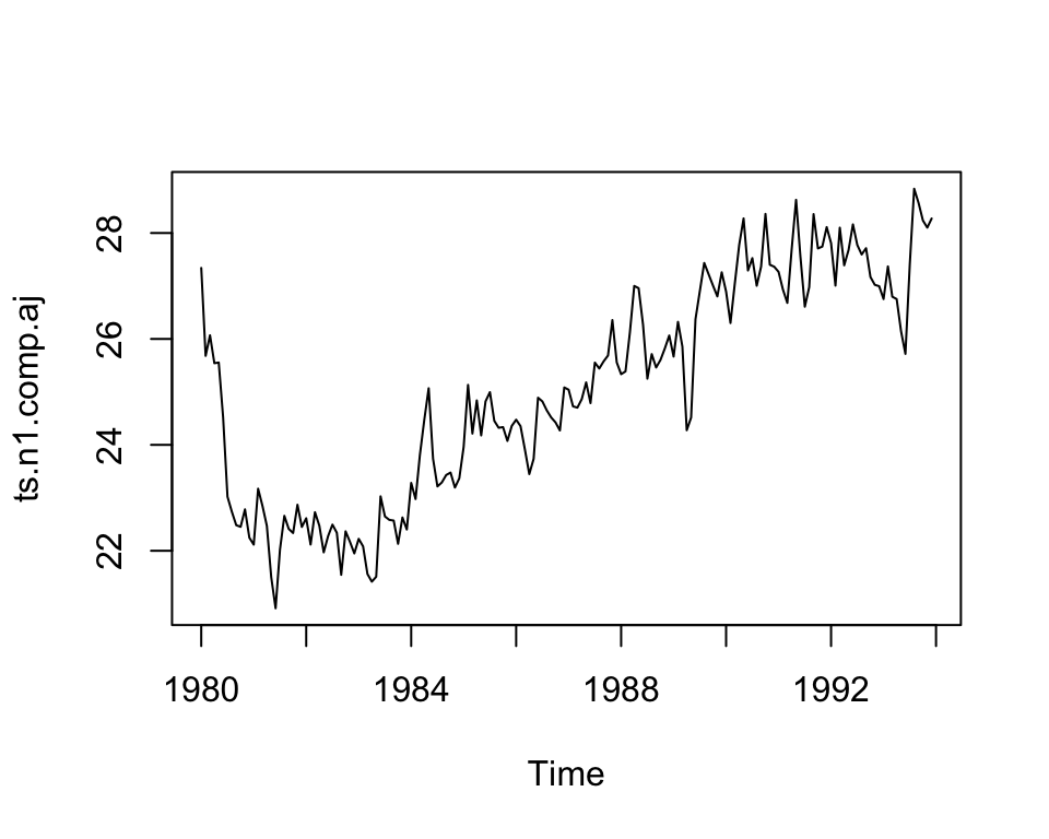
plot.ts(ts.n1)
In the second one, there seems to be seasonal variation in the number of unemployees per month: There is a peak every summer, and a trough every winter.
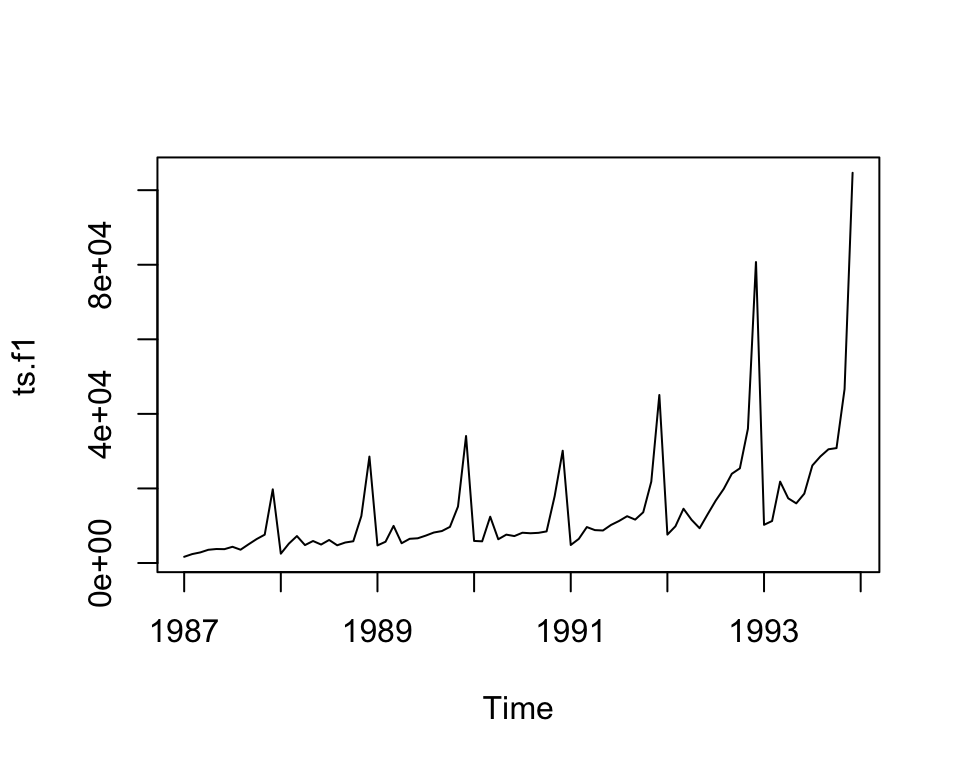
The plot for the third dataset is the following:
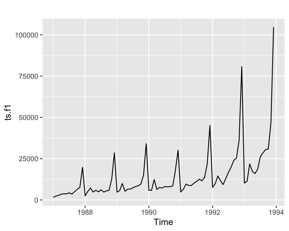
plot.ts(ts.f1)
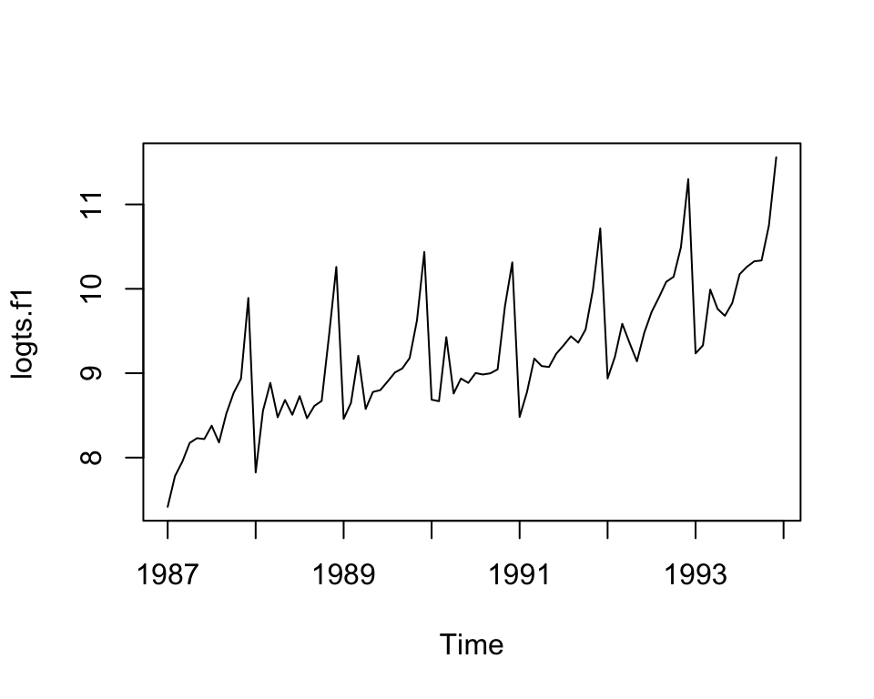
The size of the seasonal fluctuations and random fluctuations seem to increase with the level of the time series. In these cases it is reasonable to transform the time series by calculating the natural logarithm of the original data.
With one of the previously imported series (tsf1), we are fitting the model:
\[y=a+bx+cx^2\]
library(ggplot2)library(forecast)str(ts.f1)## Time-Series [1:84] from 1987 to 1994: 1665 2398 2841 3547 3753 ...mydata <-data.frame(x=1:length(ts.f1), y=tsf1)autoplot(ts.f1)
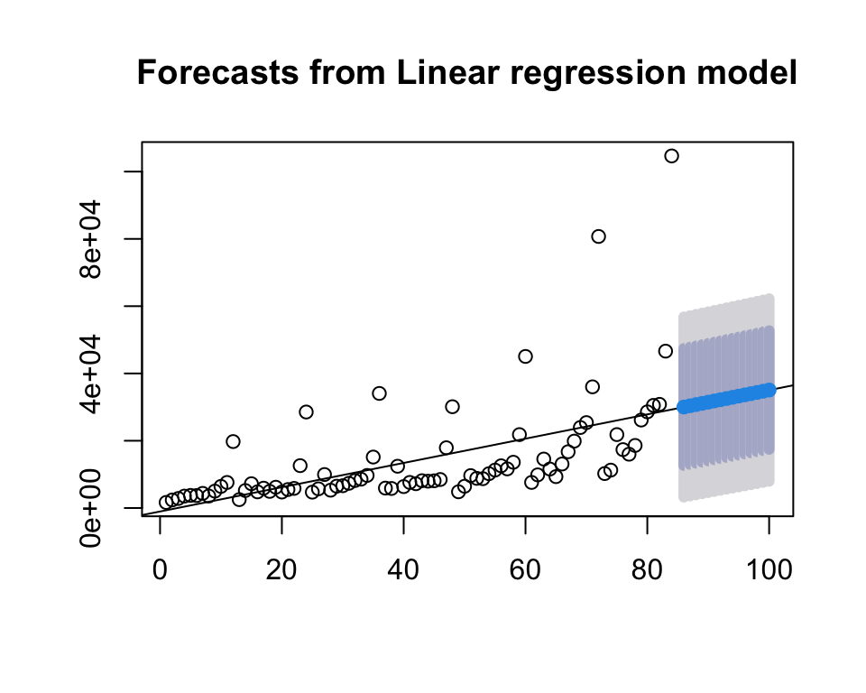
model <-lm( y ~ x , data=mydata)summary(model)## ## Call:## lm(formula = y ~ x, data = mydata)## ## Residuals:## Min 1Q Median 3Q Max ## -15084 -7058 -1498 2394 75362 ## ## Coefficients:## Estimate Std. Error t value Pr(>|t|) ## (Intercept) -1028.85 2892.21 -0.356 0.723 ## x 361.05 59.11 6.108 3.22e-08 ***## ---## Signif. codes: 0 '***' 0.001 '**' 0.01 '*' 0.05 '.' 0.1 ' ' 1## ## Residual standard error: 13140 on 82 degrees of freedom## Multiple R-squared: 0.3127, Adjusted R-squared: 0.3043 ## F-statistic: 37.31 on 1 and 82 DF, p-value: 3.222e-08prediction_model <- forecast::forecast(model, newdata =data.frame(x=86:100))plot(prediction_model)
5.2.3 Time Series Components
A time series has usually a trend component and an irregular component and, if it turns out to be a seasonal time series, a seasonal component as well.
base R: times series class named ts. too restrictive, functiones associated limited
zoo, xts packages: to represent time series
special structure for time series
many functions interestings
Exercise
Make an .rmd with a mini-tutorial on the use of the zoo and xts packages, applying them to a time series (dataset with data from Spain) that you search on the web about electricity consumption, product consumption, etc.
Hand in the homework of the time series topic.
5.2.4.1 Basic forecasting methods
We denote \(\hat{y}_{T+h\mid T}\) the value of the variable \(y\) in the time \(T+h\) based on \(y_1, \ldots, y_T\).
The residual will be computed by:
\[e_T=y_T-\hat{y}_{T}\] The forecast error is: \[e_t(T)=y_t-\hat{y}_{t}(t-T)\]
Note: It is necessary the package fpp2 to execute the code in this page.
5.2.8 Example: Temperature forecast in Malaga - Basic forecasting methods
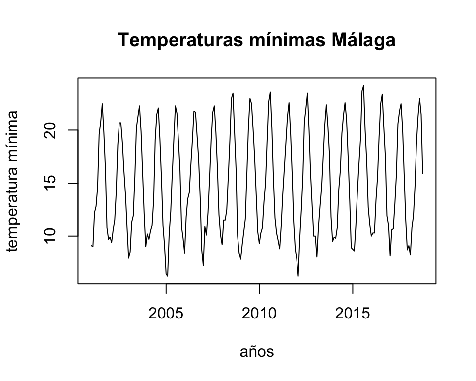
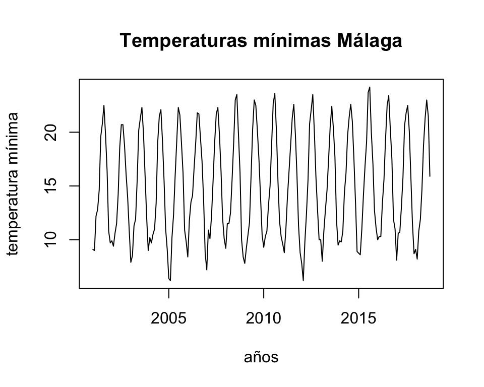
To analyse the evolution of minimum temperatures since 2001 in Malaga.
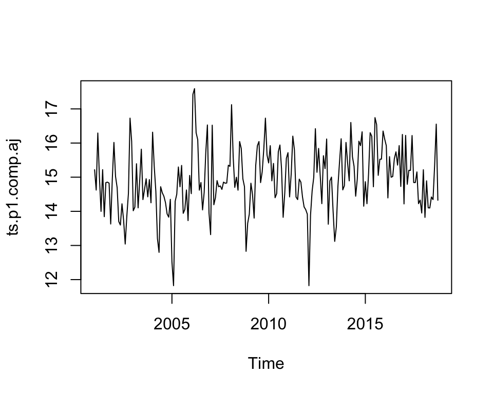
First of all we obtain a time-series object with the function ts, as our data are divided into months, we set the parameter frecuency to 12 and we indicate that we start in January 2001. After this, we draw the object obtained:
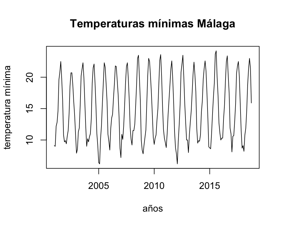
library(readr)## Warning: package 'readr' was built under R version 4.3.1temperaturas <-read_csv( here::here("data","temp.csv"))## Rows: 214 Columns: 6## ── Column specification ────────────────────────────────────────────────────────## Delimiter: ","## chr (2): fecha, indicativo## dbl (4): X1, X1_1, tm_max, tm_min## ## ℹ Use `spec()` to retrieve the full column specification for this data.## ℹ Specify the column types or set `show_col_types = FALSE` to quiet this message.ts.p1 <-ts(temperaturas$tm_min, start =c(2001, 1), frequency =12)plot.ts(ts.p1, xlab ="años", ylab ="temperatura mínima", main ="Temperaturas mínimas Málaga")
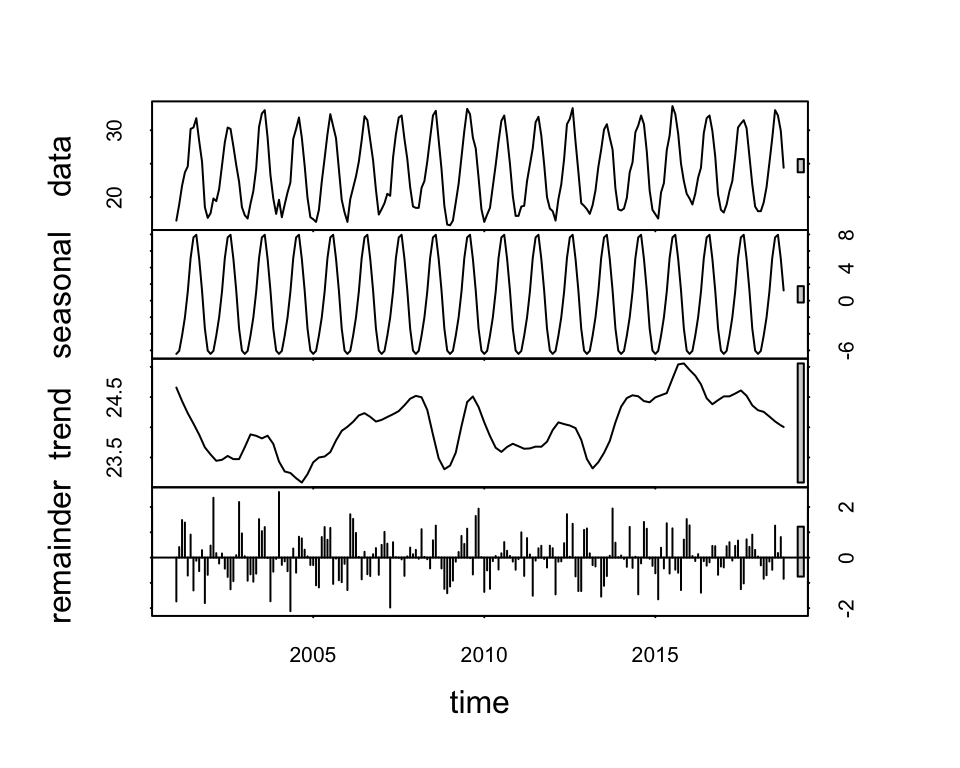
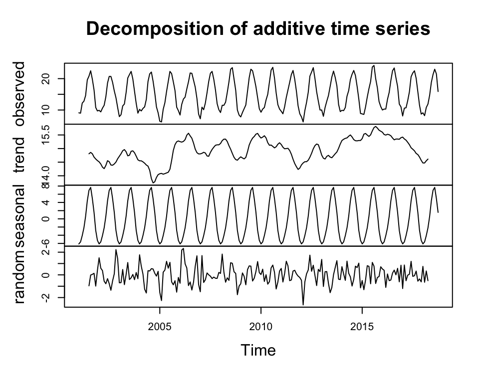
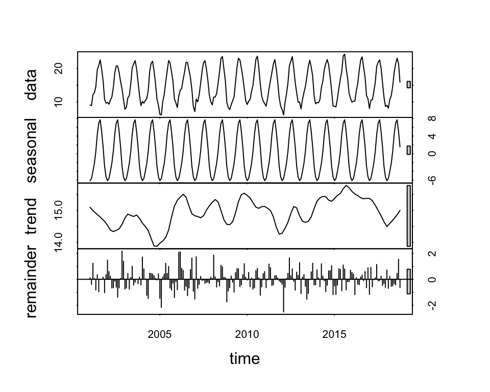
We decompose the data: Seasonal component, Trend component, Cycle component y residual.
# obtenemos una serie temporal con frecuencia 12 mesesobj.ts <-ts(na.omit(temperaturas$tm_max), frequency =12, start =c(2001, 1))# descomposedecomp <-stl(obj.ts, s.window ="periodic") # uses additive model by default# decomposing the series and removing the seasonality can be done with seasadj() within the forecast packagedeseasonal_cnt <-seasadj(decomp)plot(decomp)
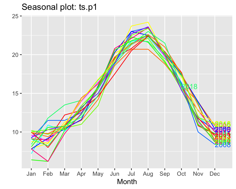
Let’s see if it is seasonal, let’s look at the data by year:
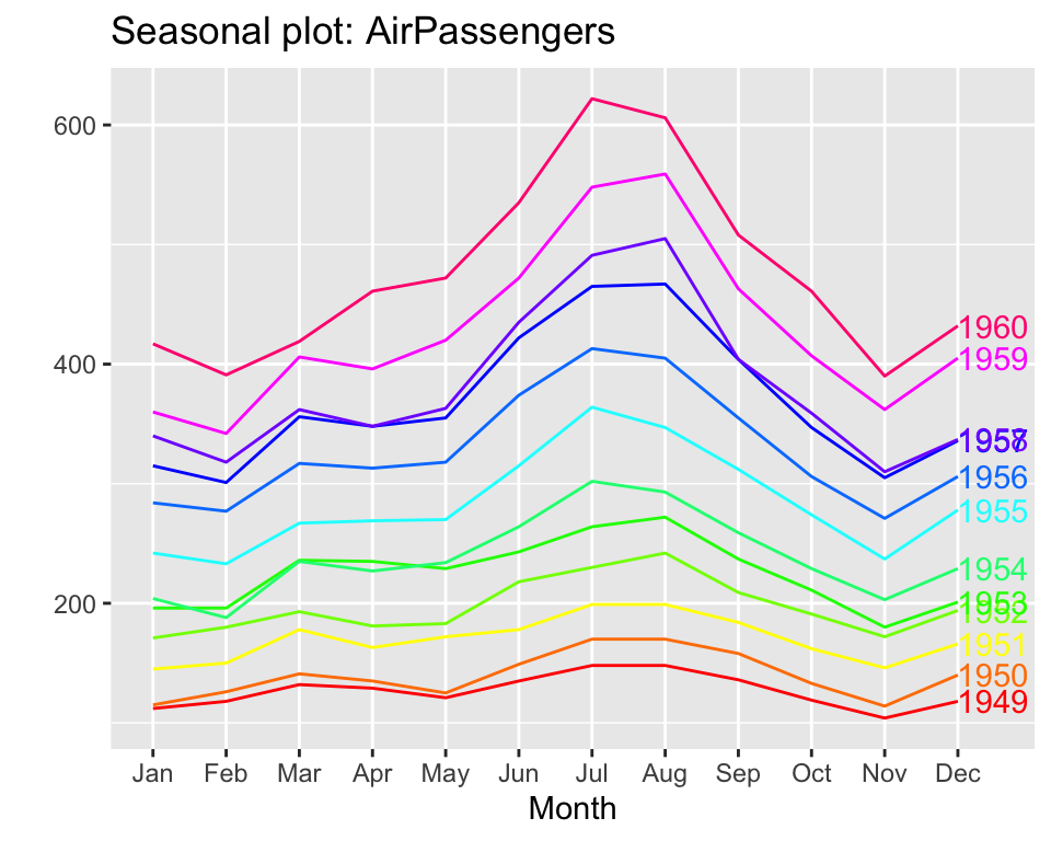
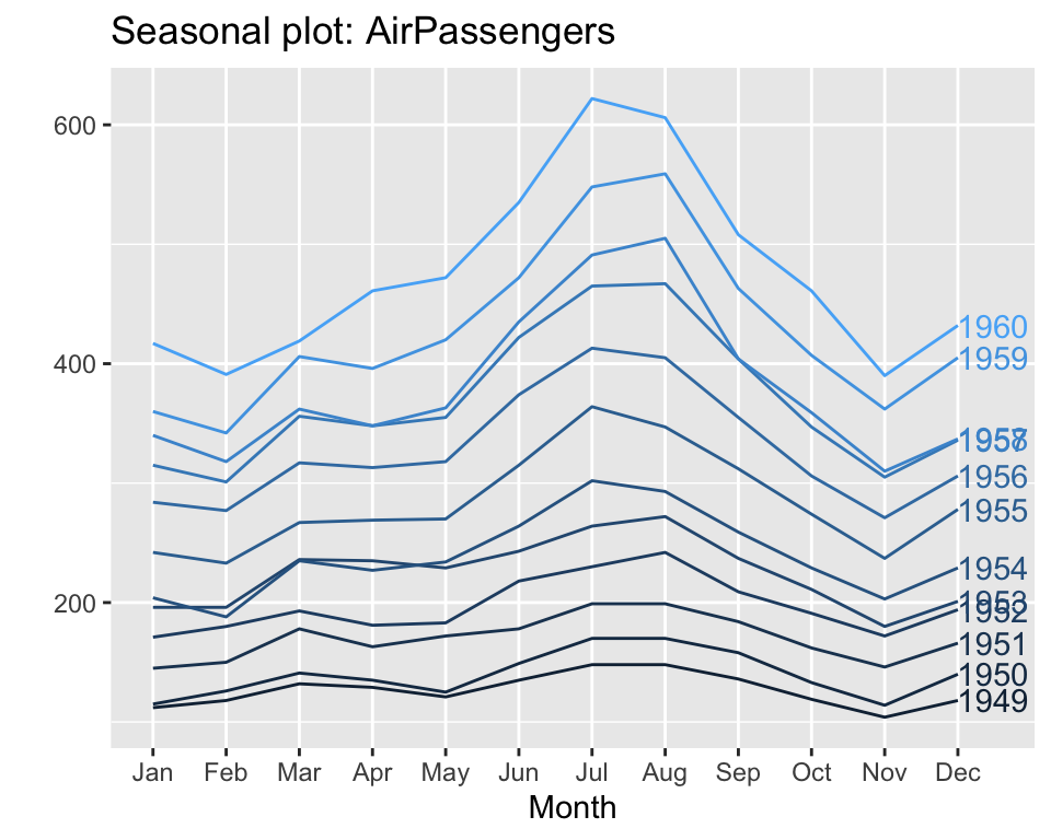
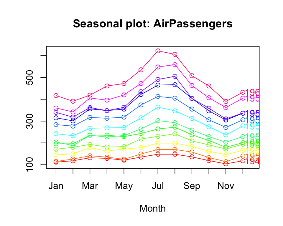
ggseasonplot(ts.p1, col =rainbow(12), year.labels =TRUE)
As we can see, all the years are identical, which indicates that the temperatures repeat annual and monthly cycles.
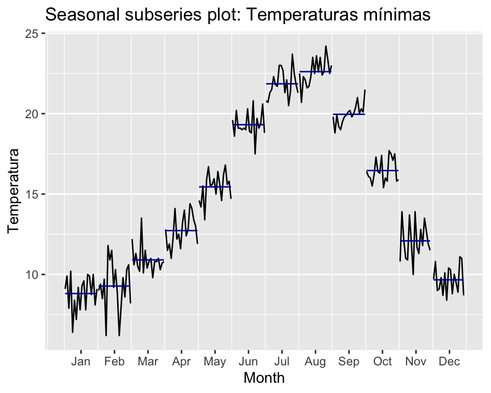
With these graphs we can see that our series is seasonal, at the beginning of the year it is down, during the year it rises and from August onwards it starts to fall. This cycle is repeated every year.
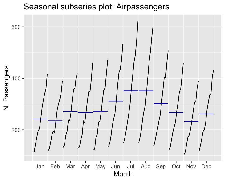
With this last graph we see the subseries by months. From it we see how each month moves in the same range. With this we confirm that it is a seasonal series.
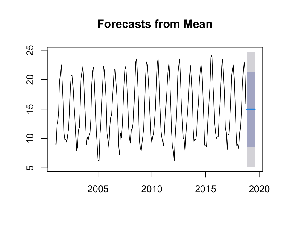
5.2.8.1 Average method
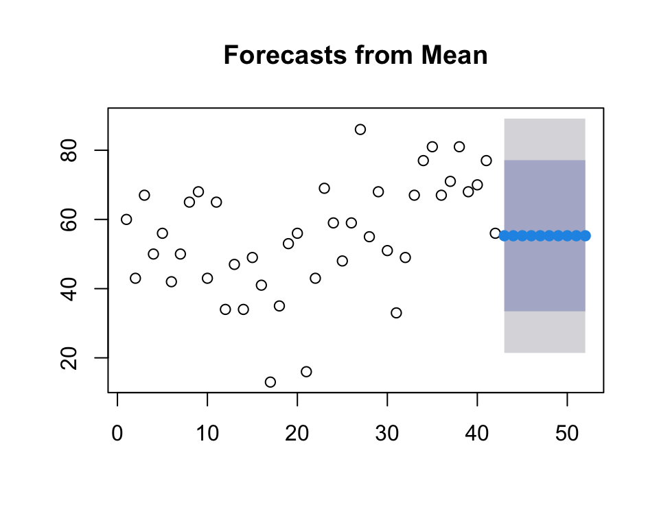
With this method we see that the prediction is basically an average.
mdata.ts.p1 <-meanf(ts.p1,10)plot(mdata.ts.p1)
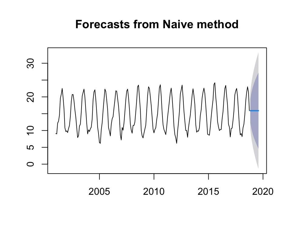
5.2.8.2 Naïve method
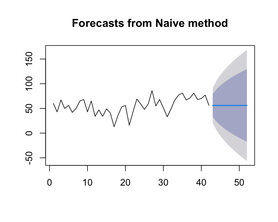
This method uses the last value of \(y_t\).
mdata.ts.p1 <-naive(ts.p1, 10)plot(mdata.ts.p1)
5.2.8.3 Seasonal naïve method
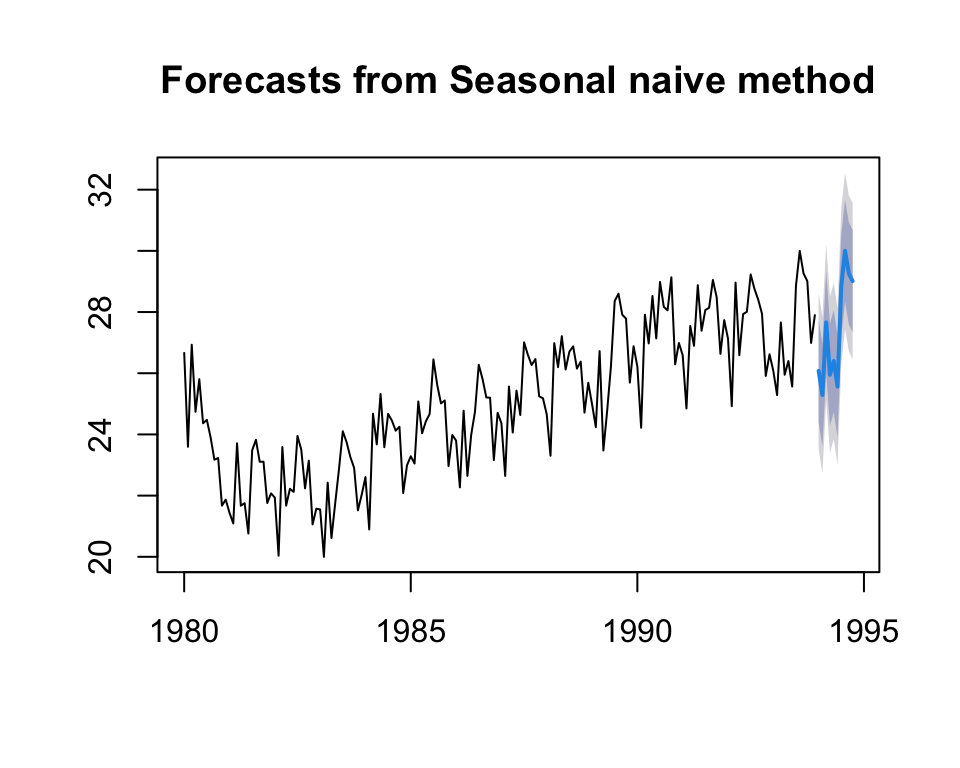
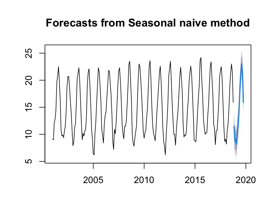
This method uses the last year to predict. As we will see in the graph, it generates what has happened in the last year.
mdata.ts.p1 <-snaive(ts.p1, 12)plot(mdata.ts.p1)
5.2.8.4 Drift method
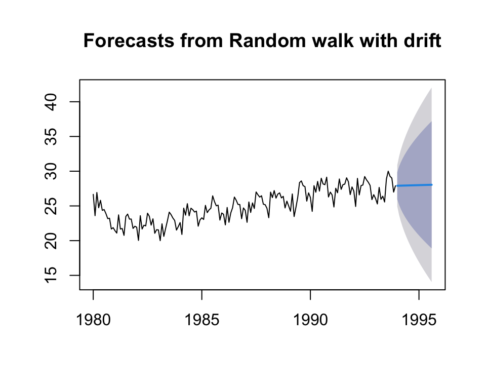
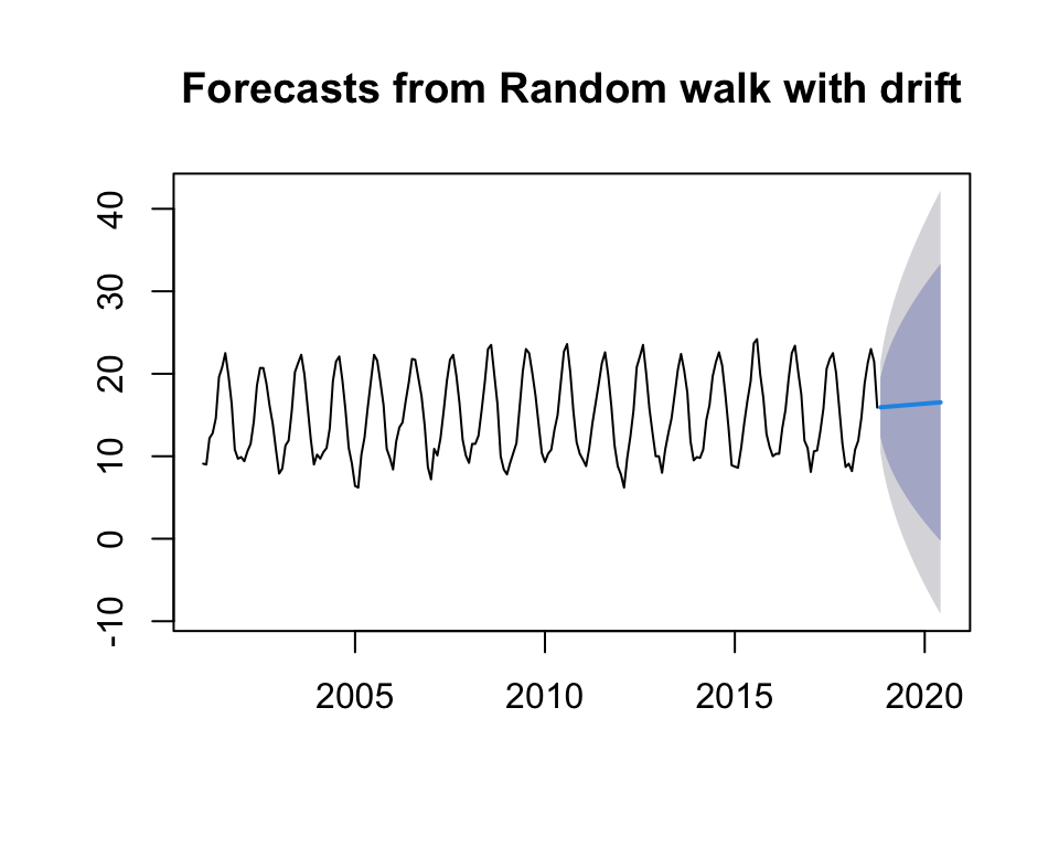
This method is based on the previous one and that the amount of change over time is set as the average change in the historical data.
My data series as I have mentioned is for minimum temperatures, so these methods are too simple to predict well what will happen with the temperature in the following years. The only model that could be used is the Seasonal naïve method which uses the last year to see what will happen next year. But we still need to use better methods.
5.3 Decomposing Time Series
Decomposing a time series means separating it into its constituent components: trend, cycles, irregular, a seasonal component and a remainder component.
If \(S_t\) is the seasonal component, \(T_t\) is the trend-cycle component, and \(R_t\) is the remainder component, we can consider an additive decomposition or a multiplicative decomposition as follows:
Addditve decomposition is adequate when the seasonal part and the trend-cycle does not vary too much.
Multiplicative decomposition is adequate when the amplitude of the seasonal part increases or decreases with the average level of the time series.
Multiplicative decomposition can be transformed into an additive one just by applying logarithms: \[\log y_t= \log S_t + \log T_t +\log R_t\]
5.3.1 Additive decomposition
We describe how decompose a time series considering additive decomposition.
Note: Multiplicative decomposition is similar, except that the subtractions are replaced by divisions.
5.3.2 Non-Seasonal Data
A non-seasonal time series consists of a trend component and an irregular component.
To estimate the trend component of a non-seasonal time series that can be described using an additive model, it is common to use a smoothing method, such as calculating the Simple Moving Average (SMA) of the time series.
The SMA() function in the TTR package is used to smooth time series data using a simple moving average:
To compute the average eliminates randomness in the data.
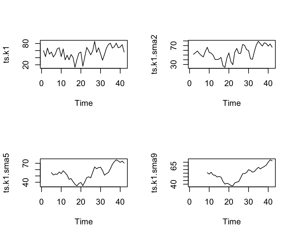
To specify the order of the simple moving average, the parameter \(n\) will be used. For example, to calculate a simple moving average of order 2, we set \(n=2\) in the SMA() function.
library("TTR")# simple moving average of order 2# applied in the first datasetdata.ts.k1 <-scan( here::here("data","ts_k1.dat"), skip =1)ts.k1 <-ts(data.ts.k1)# Applying the MA of order 2,5,9ts.k1.sma2 <-SMA(ts.k1, n =2)ts.k1.sma5 <-SMA(ts.k1, n =5)ts.k1.sma9 <-SMA(ts.k1, n =9)# Draw all the pictures togetherpar(mfrow =c(2, 2))plot.ts(ts.k1)plot.ts(ts.k1.sma2)plot.ts(ts.k1.sma5)plot.ts(ts.k1.sma9)
There still appears to be quite a lot of random fluctuations in the time series smoothed using a simple moving average of order 2.
Thus, to estimate the trend component more accurately, we might want to try smoothing the data with a simple moving average of a higher order. This takes a little bit of trial-and-error, to find the right amount of smoothing.
With MA of order 5, and order 9 the trend starts to be clearly identified in the plots.
5.3.3 Seasonal Data
A seasonal time series consists of a trend component, a seasonal component and an irregular component.
We can use the decompose function in R which estimates:
the trend-cycle component using MA \(\hat{y_t}\),
the detrended serie \(y_t-\hat{y_t}\)
the seasonal component \(S_t\), computing the average of the detrended values for that season,
the random components \(R_t=y_t-\hat{y_t}-S_t\).
To compute the detrended serie in additive decomposition: \(y_t-T_t =S_t+R_t\)
Given the time series ts.n1, we will decompose the time serie using the following:
As we have explained, if you have a seasonal time series that can be described using an additive model, you can seasonally adjust the time series by estimating the seasonal component, and subtracting the estimated seasonal component from the original time series.
The seasonal variation has been removed from the seasonally adjusted time series. The seasonally adjusted time series now just contains the trend component and an irregular component.
5.3.5 Example: Temperature forecast in Malaga - Decomposing Time Series
We have seen that the time series we use is seasonal so we are going to use the method of Additive decomposition.
5.3.5.1 Additive decomposition
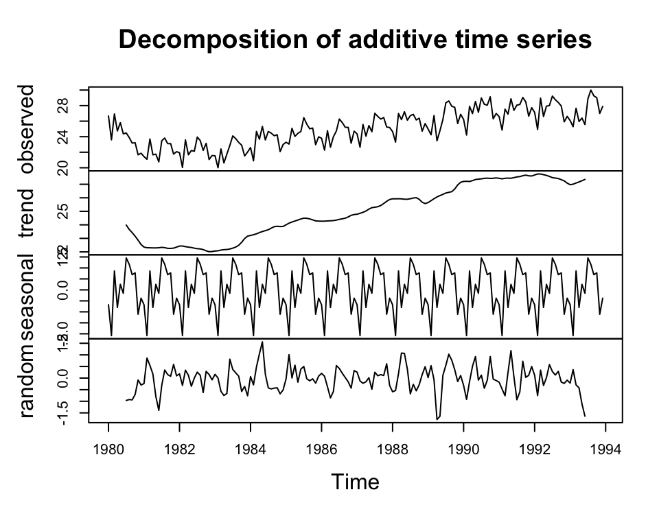
A seasonal time series consists of a trend component, a seasonal component and an irregular component. To decompose it we are going to use decompose.
# we decompose the time series and draw itts.p1.comp <-decompose(ts.p1)plot(ts.p1.comp)
5.3.6 Seasonal Adjusting
If we have a seasonal time series that can be described using an additive model, we can seasonally adjust the time series by estimating the seasonal component and subtracting the estimated seasonal component from the original time series.
Exponential Smoothing considers weigths to the values of the variables: weighted averages of past observations. The weights decrease exponentially for distant values.
The parameter \(\alpha\) controls the rates at which the weights decrease. The weights decrease exponentially and this is the reason of the name of the method.
\(\alpha\) has values between 0 and 1.
\(\alpha\) close to 0, more important are the longer observations - slow learning (past observations have a large influence on forecasts).
\(\alpha\) close to 1, more important the more recent observation s- fast learning (that is, only the most recent values influence the forecasts).
With \(\alpha=0\) or \(\alpha=1\) we have the extreme cases.
If you have a time series that can be described using an additive model with constant level (no clear trend) and no seasonality, you can use simple exponential smoothing to make short-term forecasts.
The simple exponential smoothing method provides a way of estimating the level at the current time point.
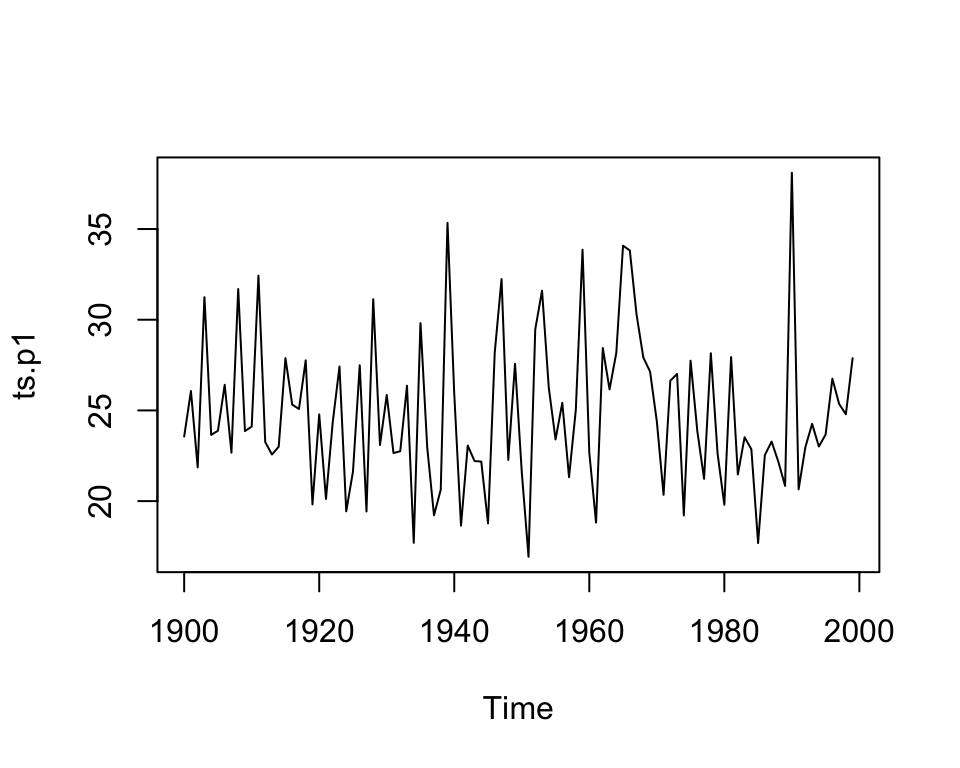
The file ts_p1.dat contains total annual snowfall for a city.
alpha: Smoothing is controlled by this parameter; the value of alpha lies between 0 and 1 (close to 0 mean that little weight is placed on the most recent observations when making forecasts of future values).
beta=FALSE: the function will do exponential smoothing.
gamma=FALSE: a non-seasonal model is fitted.
seasonal: additive by default or multiplicative seasonal model.
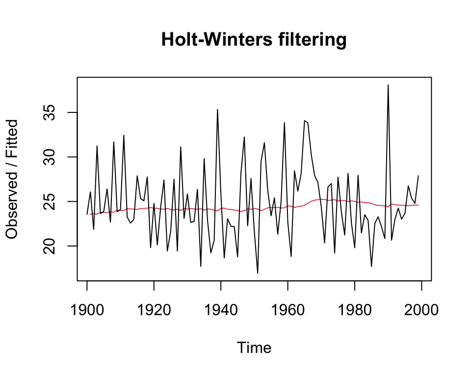
The output of HoltWinters() tells us that the estimated value of the alpha parameter is about 0.024. This is very close to zero, telling us that past observations have more influence on forecasts.
plot(ts.p1.forecasts)
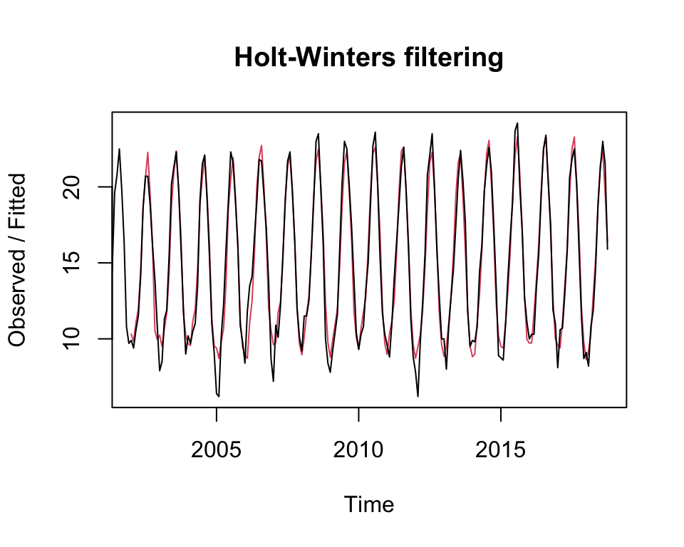
The plot shows the original time series in black, and the forecasts of these values as a red line. The time series of forecasts is much smoother than the time series of the original data here.
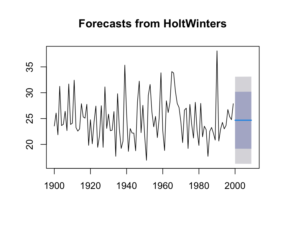
plot(forecast(ts.p1.forecasts))
The function forecast predicts the value as the previous plot shows.
As a measure of the accuracy of the forecasts, we can calculate the sum of squared errors for the in-sample forecast errors, that is, the forecast errors for the time period covered by our original time series. The sum-of-squared- errors is stored in a named element of the list variable ts.p1.forecasts called “SSE”, so we can get its value by typing:
ts.p1.forecasts$SSE## [1] 1828.855
Finally, we try with different values of \(\alpha\) and the errors are computed:
We can make forecasts for further time points by using the forecast.HoltWinters function in the R forecast package.
require("forecast")library("forecast")
When using the forecast.HoltWinters function, as its first argument (input), you pass it the predictive model that you have already fitted using the HoltWinters function.
You specify how many further time points you want to make forecasts for by using the “h” parameter in forecast.HoltWinters().
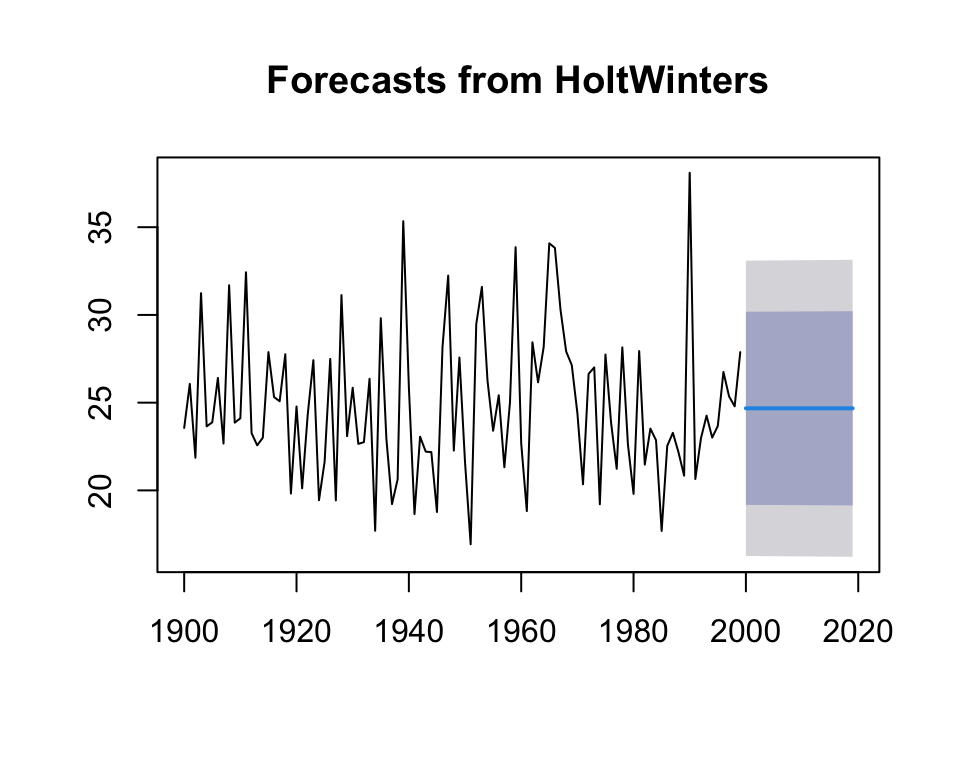
The forecast for a year, a 80% prediction interval for the forecast, and a 95% prediction interval for the forecast.
Plotting the predictions:
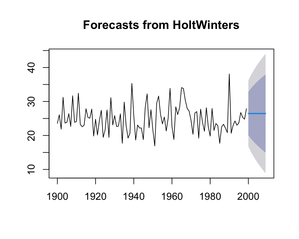
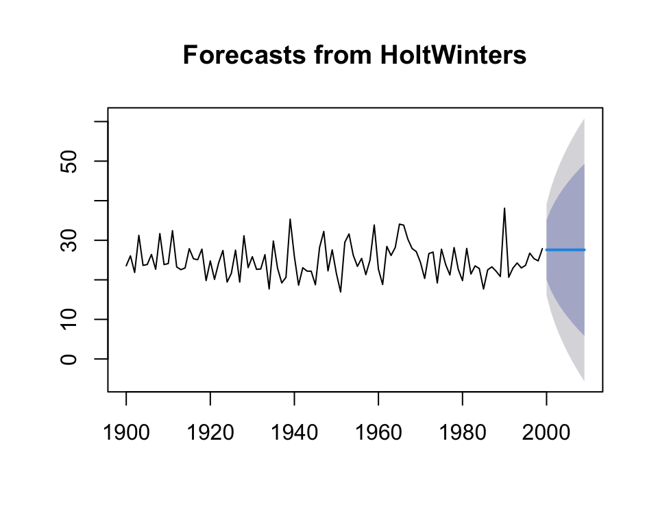
forecast:::plot.forecast(ts.p1.forecasts2)
The forecasts for 2000-2020 are plotted as a blue line, the 80% prediction interval as a dark blue shaded area, and the 95% prediction interval as a grey shaded area.
Forecast errors
Forecast errors are stored in the element residuals.
If the predictive model cannot be improved upon, there should be no correlations between forecast errors for successive predictions.
If there are correlations between forecast errors for successive predictions, it is likely that the simple exponential smoothing forecasts could be improved upon by another forecasting technique.
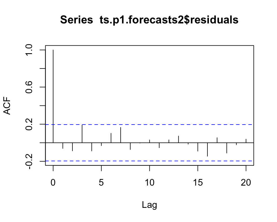
To figure out whether this is the case, we can obtain a correlogram of the in-sample forecast errors. We can calculate a correlogram of the forecast errors using the acf function in R.
acf computes (and plots, by default) the estimation of the autocovariance or AutoCorrelation Function (ACF).
The autocorrelation at lag 3 is just touching the significance bounds (significant evidence for non-zero correlations).
To test whether there is significant evidence for non-zero correlations at lags, we can carry out a Ljung- Box test. This can be done in R using the Box.test function.
Box.test(ts.p1.forecasts2$residuals, lag =20, type ="Ljung-Box")## ## Box-Ljung test## ## data: ts.p1.forecasts2$residuals## X-squared = 17.401, df = 20, p-value = 0.6268
The p-value is 0.6, so there is little evidence of non-zero autocorrelations in the in-sample forecast errors at lags 1-20.
5.3.10 ACF test
ACF (AutoCorrelation Function):
Purpose: The ACF is used to study and visualize the autocorrelation in a time series. Autocorrelation measures the relationship between a data point and its past lags (previous observations in the series). It helps you understand the patterns, cycles, and seasonality in the data.
How it works: The ACF computes and plots the autocorrelation coefficients for different lags. It shows the strength and direction (positive or negative) of the correlation between each observation and its lags.
Interpretation: ACF can help you identify significant lags in the data, which can inform the choice of lag order in models like ARIMA (see below). Significant lags may indicate seasonality or other patterns in the data.
In an ACF (AutoCorrelation Function) test, if you observe a significant autocorrelation at lag 3, it means that there is a statistically meaningful relationship between data points that are separated by a lag of 3 time periods (lags). Here’s what this implies:
Lag 3 Autocorrelation: At lag 3, the ACF measures the correlation between the current data point and the data point that is three time periods (time steps) in the past. A positive autocorrelation suggests that as the current data point increases, the data point at lag 3 also tends to increase, and vice versa for a negative autocorrelation.
Significance: When we say that the autocorrelation at lag 3 is “significant,” it means that the correlation is unlikely to have occurred by random chance. In other words, the autocorrelation is strong enough to be considered a real relationship in the data.
Interpretation: The significance of a lag in the ACF can provide insights into potential patterns or seasonality in the time series. For example, a significant positive autocorrelation at lag 3 might suggest that the time series exhibits a repeating pattern or cycle with a length of 3 time periods.
Modeling: When building time series models like ARIMA, the presence of significant lags in the ACF can inform the choice of model parameters (e.g., the autoregressive order, denoted as ‘p’ in ARIMA) to capture these relationships and patterns.
In summary, a significant autocorrelation at lag 3 in the ACF suggests that there is a meaningful relationship between data points separated by a lag of 3 time periods, which can be indicative of repeating patterns or seasonality in the time series. It’s an important finding when analyzing and modeling time series data.
5.3.11 Example: Temperature forecast in Malaga - Exponential Smoothing
Analyse the evolution of minimum temperatures since 2001 in Malaga with the methods seen in this document. Malaga with the methods seen in this document**.
We obtain a time-series object with the ts function. data are divided into months, the parameter frequency is set to 12 and we indicate that we start in January 2001. After this, we draw the object:
library(readr)temperaturas <-read_csv( here::here("data","temp.csv"))## Rows: 214 Columns: 6## ── Column specification ────────────────────────────────────────────────────────## Delimiter: ","## chr (2): fecha, indicativo## dbl (4): X1, X1_1, tm_max, tm_min## ## ℹ Use `spec()` to retrieve the full column specification for this data.## ℹ Specify the column types or set `show_col_types = FALSE` to quiet this message.ts.p1 <-ts(temperaturas$tm_min, start =c(2001, 1), frequency =12)plot.ts(ts.p1, xlab ="años", ylab ="temperatura mínima", main ="Temperaturas mínimas Málaga")
Forecasts using Exponential Smoothing
Exponential Smoothing considers weights on variable values: weighted averages of past observations. The weights decrease exponentially for distant values.
5.3.11.1 Simple Exponential Smoothing
alpha parameter of Holt-Winters Filter.
beta parameter of Holt-Winters Filter. If set to FALSE, the function will do exponential smoothing.
gamma parameter used for the seasonal component. If set to FALSE, an non-seasonal model is fitted.
Looking at these parameters we have to assemble a model with beta=FALSE as we want exponential smoothing.
The graph shows the original time series in black, and forecasts of these values as a red line. The forecast time series is very close to the original data.
We now draw the forecast using forecast.
plot(forecast(ts.p1.forecasts))
As we can see it fits quite well with what is happening in recent years.
As we can see there is not much difference between the first model and the other 2 created later, so the alpha value generated by the first model is the optimal one. We can see that the higher the alpha value, the narrower the fixed values, and the gamma values increase along with alpha.
5.3.12 Forecasting using forecast package
When we use the forecast.HoltWinters function, as the first argument, it is passed the predictive model that we have already set using the HoltWinters function.
To specify how many additional time points we want to predict, we use the parameter “h”.
The prediction for the next 2 years is:
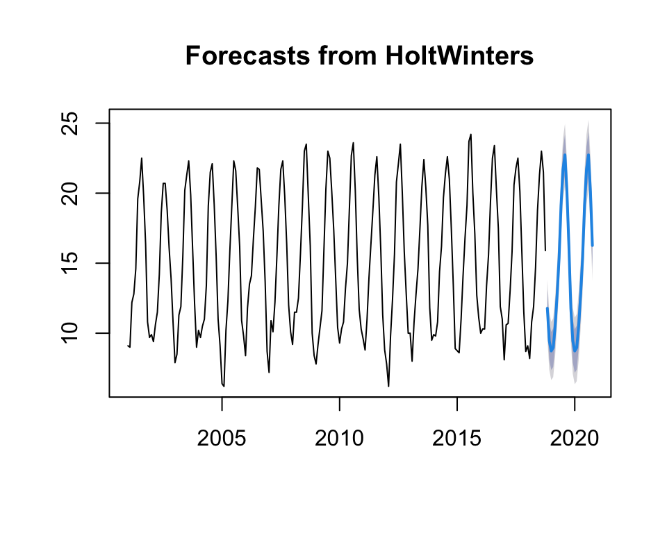
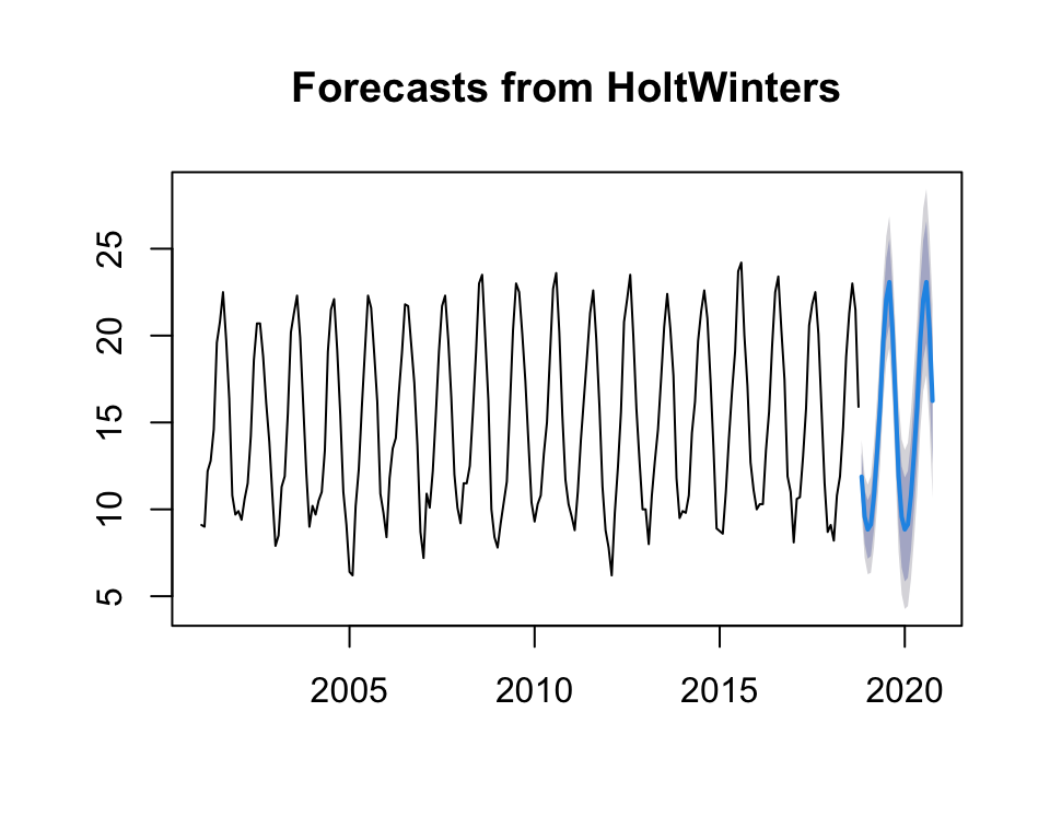
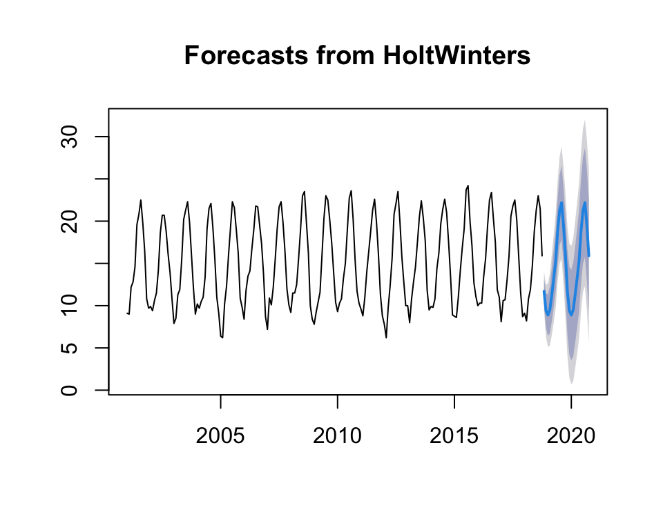
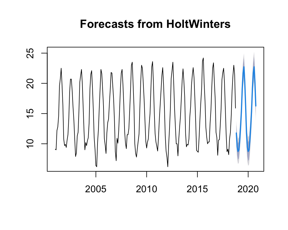
# we indicate the parameter h=24 for 2 years, as we have the time series by monthsts.p1.forecasts2 <- forecast:::forecast.HoltWinters(ts.p1.forecasts, h =24)ts.p1.forecasts2## Point Forecast Lo 80 Hi 80 Lo 95 Hi 95## Nov 2018 11.782247 10.448881 13.11561 9.743039 13.82146## Dec 2018 9.451858 8.105265 10.79845 7.392421 11.51129## Jan 2019 8.732563 7.372871 10.09225 6.653094 10.81203## Feb 2019 8.970131 7.597467 10.34279 6.870822 11.06944## Mar 2019 10.503103 9.117587 11.88862 8.384139 12.62207## Apr 2019 12.740432 11.342183 14.13868 10.601995 14.87887## May 2019 15.344559 13.933692 16.75543 13.186823 17.50229## Jun 2019 19.151450 17.728075 20.57482 16.974587 21.32831## Jul 2019 21.708406 20.272634 23.14418 19.512582 23.90423## Aug 2019 22.732955 21.284891 24.18102 20.518333 24.94758## Sep 2019 20.136368 18.676116 21.59662 17.903106 22.36963## Oct 2019 16.261252 14.788913 17.73359 14.009504 18.51300## Nov 2019 11.782247 10.250481 13.31401 9.439613 14.12488## Dec 2019 9.451858 7.908565 10.99515 7.091594 11.81212## Jan 2020 8.732563 7.177827 10.28730 6.354800 11.11032## Feb 2020 8.970131 7.404038 10.53622 6.574998 11.36526## Mar 2020 10.503103 8.925733 12.08047 8.090724 12.91548## Apr 2020 12.740432 11.151866 14.32900 10.310930 15.16993## May 2020 15.344559 13.744875 16.94424 12.898054 17.79106## Jun 2020 19.151450 17.540725 20.76217 16.688058 21.61484## Jul 2020 21.708406 20.086715 23.33010 19.228243 24.18857## Aug 2020 22.732955 21.100371 24.36554 20.236134 25.22978## Sep 2020 20.136368 18.492964 21.77977 17.622999 22.64974## Oct 2020 16.261252 14.607099 17.91541 13.731443 18.79106
forecast:::plot.forecast(ts.p1.forecasts2)
The forecasts for the next 2 years are represented as a blue line, the 80% prediction interval as a dark grey shaded area and the 95% prediction interval as a grey shaded area.
Forecast errors
Errors are stored in residuals.
If the model cannot be improved, there should be no correlations between forecast errors for successive predictions.
If there are correlations between forecast errors for successive predictions, it is likely that the predictions can be improved with another technique.
To find out which is the case, we can obtain a correlation of the errors. We can calculate it using the acf function. acf calculates the estimate of the autocovariance or autocorrelation function (ACF).
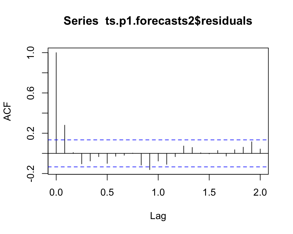
Let’s see what happens, we use acf with residuals and lag max 24.
# na.action, to take or not to take into account the NA valuesacf(ts.p1.forecasts2$residuals, na.action = na.pass, lag.max =24)
We performed a Ljung Box text to see if there is significant evidence of non-zero correlations in the lag.
Box.test(ts.p1.forecasts2$residuals, lag =24, type ="Ljung-Box")## ## Box-Ljung test## ## data: ts.p1.forecasts2$residuals## X-squared = 41.723, df = 24, p-value = 0.01386
As we can see, the p-value is 0.01, which tells us that there is evidence of autocorrelations other than 0.
Note: The ACF (AutoCorrelation Function) chart is used to identify non-stationary time series. Stationary: if the ACF is rapidly declining
6 ARIMA models versus Holt-Winters models
The difference between exponential smoothing models and ARIMA models is that the former are based on a description of the trend and seasonality of the data, while ARIMA models study the autocorrelations of the data.
6.1 Characteristics
ARIMA (AutoRegressive Integrated Moving Average): - ARIMA decomposes a time series into three components: AutoRegressive (AR), Integrated (I), and Moving Average (MA). - ARIMA is particularly effective when dealing with stationary time series data, meaning that the statistical properties of the data do not change over time.
Holt-Winters: - Holt-Winters is a triple exponential smoothing method that decomposes a time series into three components: level, trend, and seasonality. - Holt-Winters is designed for time series data with trend and seasonality, making it a good choice for data that exhibits systematic patterns over time.
6.1.1 Stationarity
A stationary time series is one where the statistical properties of the data do not change over time, specifically with respect to time-dependent moments like mean, variance, and covariance.
 a. Constant Mean: The mean (average) of the time series data remains roughly constant over time.
b. Constant Variance: The variance (spread or dispersion) of the data remains roughly constant over time.
c. Constant Autocovariance: The autocovariance (covariance between data points at different time lags) remains roughly constant over time.
A time series is said to be stationary when it does not depend on the instant of observation (white noise series).
In a stationary time series, the behavior of the data is not influenced by when the data was collected. This means that the patterns and characteristics of the data are consistent regardless of the time at which you look at it.
White noise is a specific type of stationary time series where each data point is independently and identically distributed with a constant mean and constant variance. In other words, white noise is a stationary time series with no systematic patterns, trends, or correlations between data points.
If a series has a trend or stationarity it is not stationary.
A time series that has a cyclical component is stationary.
When a time series it exhibits these stationary characteristics, and it is often easier to analyze and model because the statistical properties do not change with time.
This is an important assumption in many time series analysis techniques, such as autoregressive integrated moving average (ARIMA) modeling.
If a time series is not stationary, it may require transformation (e.g., differencing) to make it stationary before applying certain analytical methods.
Stationarity with ARIMA?: - ARIMA models require that the time series be made stationary, often through differencing. - ARIMA is suitable for data with or without seasonality as long as it can be made stationary.
Stationarity with Holt-Winters?: - Holt-Winters can handle non-stationary data but is especially effective for time series with seasonality and trends.
6.1.2 Stationary?
6.1.2.1 Example
From a dataset from sales, we check for stationarity using the Augmented Dickey-Fuller (ADF) test and fit an ARIMA model to the stationary data.
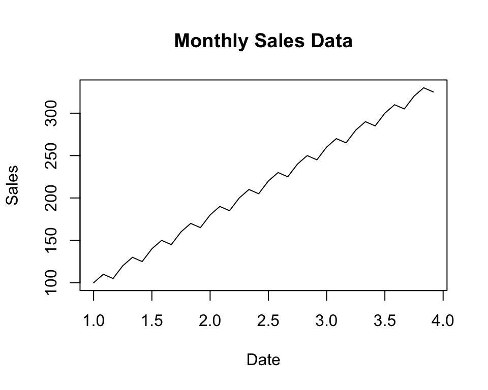
# Create a simple example datasetdate <-seq(as.Date("2020-01-01"), by ="1 month", length.out =36)sales <-c(100, 110, 105, 120, 130, 125, 140, 150, 145, 160, 170, 165,180, 190, 185, 200, 210, 205, 220, 230, 225, 240, 250, 245,260, 270, 265, 280, 290, 285, 300, 310, 305, 320, 330, 325)# Create a data framesales_data <-data.frame(Date = date, Sales = sales)# Save the data to a CSV filelibrary(tseries)library(forecast)# Convert the date column to a date object (adjust column name as needed)sales_data$Date <-as.Date(sales_data$Date)# Create a time series objectsales_ts <-ts(sales_data$Sales, frequency =12) # Assuming monthly data# Plot the time seriesplot(sales_ts, main ="Monthly Sales Data", xlab ="Date", ylab ="Sales")
# Check for stationarityadf_test <-adf.test(sales_ts)## Warning in adf.test(sales_ts): p-value smaller than printed p-valueif (adf_test$p.value <0.05) {cat("The time series is stationary.\n")} else {cat("The time series is not stationary. You may need to difference it.\n")}## The time series is stationary.
6.1.3 ADF test
ADF (Augmented Dickey-Fuller) Test:
Purpose: The ADF test is used to determine whether a time series is stationary or non-stationary. Stationarity is a critical assumption in time series modeling because many time series methods, like ARIMA, require data to be stationary.
How it works: The ADF test compares the observed data to a null hypothesis that the data has a unit root (non-stationary). It tests whether differencing the data (removing trends) makes it stationary.
Interpretation: The ADF test provides a test statistic and a p-value. If the p-value is less than a chosen significance level (e.g., 0.05), you can reject the null hypothesis and conclude that the data is stationary. If the p-value is greater, you may not be able to conclude stationarity.
The adf.test function will perform the ADF test on the sales_ts time series data. The results will include statistics and a p-value.
The p-value is a critical indicator to determine whether the time series is stationary. If the p-value is less than your chosen significance level (e.g., 0.05), you can conclude that the time series is stationary.
print(adf_test)## ## Augmented Dickey-Fuller Test## ## data: sales_ts## Dickey-Fuller = -1.6224e+15, Lag order = 3, p-value = 0.01## alternative hypothesis: stationary
p-value: The p-value is 0.01.
This indicates that the stationarity of the time series is strong, and it doesn’t require additional differencing.
Alternative hypothesis: The alternative hypothesis is “stationary.”
The p-value is the key component to determine stationarity. In this case, the p-value is 0.01, which is less than the commonly chosen significance level of 0.05. When the p-value is less than your chosen significance level, you can reject the null hypothesis that the time series is non-stationary. Therefore, based on the low p-value of 0.01, you can conclude that your time series is stationary.
The “Lag order” value of 3 in the Augmented Dickey-Fuller (ADF) test results indicates the number of lags used in the test to account for potential autocorrelation in the time series data. Specifically, it represents the number of past observations (time steps) that are considered when testing for stationarity.
In this case, a lag order of 3 means that the test includes three lagged differences, which can be indicative of repeating patterns or seasonality in the time series. s
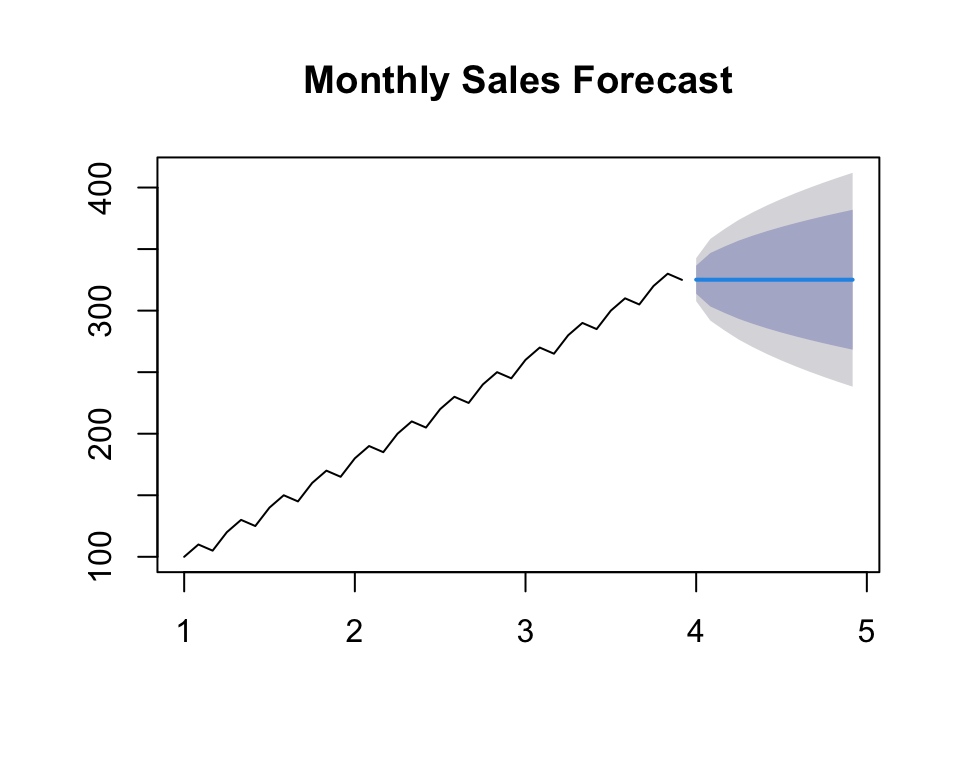
After fitting the model, we generate a forecast for future sales and plot the forecasted values.
# Fit an ARIMA model (adjust the order based on your analysis)arima_model <-arima(sales_ts, order =c(1, 1, 1))# Print model summarysummary(arima_model)## ## Call:## arima(x = sales_ts, order = c(1, 1, 1))## ## Coefficients:## ar1 ma1## -0.3552 1.0000## s.e. 0.1692 0.0792## ## sigma^2 estimated as 77.43: log likelihood = -127.21, aic = 260.42## ## Training set error measures:## ME RMSE MAE MPE MAPE MASE ACF1## Training set 4.232632 8.676369 5.934374 2.135967 3.156221 0.6020379 -0.5265618# Forecast future sales (adjust the number of periods as needed)forecast_periods <-12# Number of months to forecastsales_forecast <-forecast(arima_model, h = forecast_periods)# Plot the forecastplot(sales_forecast, main ="Monthly Sales Forecast")
# Print the forecasted valuessales_forecast$mean## Jan Feb Mar Apr May Jun Jul Aug## 4 325.1436 325.0926 325.1107 325.1043 325.1066 325.1058 325.1060 325.1059## Sep Oct Nov Dec## 4 325.1060 325.1060 325.1060 325.1060
6.1.4 Forecasting Approaches
ARIMA: - ARIMA models forecast future values based on past values, their lags, and moving averages of past forecast errors. - It models the autocorrelation between observations and their lags.
Holt-Winters: - Holt-Winters models account for three components: level, trend, and seasonality. - It uses a weighted average of these components to make forecasts and is particularly well-suited for data with strong seasonality.
6.1.5 Complexity Models
ARIMA: - ARIMA models are relatively simpler, as they involve setting orders for the AR, I, and MA components. - They can be adjusted by varying the orders (p, d, q) (see below).
Holt-Winters: - Holt-Winters models are more complex due to the triple exponential smoothing approach. - They require setting parameters for level, trend, and seasonality, and potentially smoothing parameters.
6.1.6 Use Cases
ARIMA: - ARIMA is suitable for modeling time series data without strong seasonality, such as financial data or stock prices. - It is effective when the main focus is capturing lags and autocorrelation.
Holt-Winters: - Holt-Winters is ideal for data with clear seasonal patterns, like monthly sales, quarterly economic data, or daily weather observations. - It is particularly well-suited for forecasting when seasonality and trends are prominent.
In practice, the choice between ARIMA and Holt-Winters depends on the characteristics of your time series data.
It’s important to analyze your data and determine whether it exhibits seasonality, trends, and stationarity, and then choose the method that best fits those characteristics.
Additionally, hybrid models, which combine ARIMA and Holt-Winters components, can also be used for more complex time series data.
6.2 ARIMA models
ARIMA is a popular time series forecasting method used to model and predict data that has temporal dependencies.
As we have already seen, the name ARIMA comes from AutoRegressive Integrated Moving Average.
AR: the study variable is analysed using the above values (lag).
This component models the relationship between the current observation and a specified number of past observations. It captures the influence of past values on the present value. In ARIMA, this parameter is denoted as ‘p.’
MA: the regression error is a linear combination of current and past values of the signal.
This component represents the number of differences needed to make the time series stationary. Differencing is the process of subtracting an observation from a lagged observation. In ARIMA, this parameter is denoted as ‘d.’
I: replaces the value of the variable by the difference between the values and the previous values (one or more times).
This component models the relationship between the current observation and a linear combination of past forecast errors. It accounts for the influence of past forecast errors on the present value. In ARIMA, this parameter is denoted as ‘q.’
The combination of these three components (AR, I, and MA) determines the order of the ARIMA model, which is written as ARIMA(p, d, q).
ARIMA models can be obtained following the Box-Jenkins method.
6.2.1 Examples
6.2.1.1 ARIMA(1, 0, 0)
Let’s say we have monthly sales data for a store. To apply a simple ARIMA(1, 0, 0) model, we are using only the autoregressive component.
AR component (p): 1
No differencing (d): 0
No moving average (q): 0
The model obtained will be:
\[Y_t =\phi_1 \cdot Y_{t−1} +C+ε_t\] This means that the current observation depends only on the previous observation with coefficient \(\phi_1\).
This ARIMA model is relatively simple, and the forecast is based mainly on the previous observation.
library(forecast)# Generate a simple example time seriessales_data <-c(100, 110, 105, 120, 130)# Create an ARIMA(1,0,0) modelarima_model <-arima(sales_data, order =c(1, 0, 0))# phi and C: arima_model$coef## ar1 intercept ## 0.504016 113.577998# Forecast future sales (adjust the number of periods as needed)forecast_periods <-3sales_forecast <-forecast(arima_model, h = forecast_periods)# Print the forecasted valuessales_forecast$mean## Time Series:## Start = 6 ## End = 8 ## Frequency = 1 ## [1] 121.8549 117.7497 115.6806
In this example, we used only the autoregressive component to capture the relationship between the current sales and the previous month’s sales.
6.2.1.2 ARIMA(0, 1, 1)
Now, let’s consider a more complex ARIMA model with differencing and moving average components:
AR component (p): 0
One level of differencing (d): 1
to make the time series stationary
Moving Average component (q): 1
to capture the influence of past forecast errors
The model obtained will be:
\[Y_t =Y_{t−1} + \phi_1 \cdot ε_{t-1} +ε_t\] Coeficient \(\phi_1\) is the coeficient of the MA.
This ARIMA(0,1,1) model implies that future observations \(Y_t\) depend on past observations \(Y_{t-1}\) and a moving average component of order 1 \(\phi_1 \cdot ε_{t-1}\).
The first order differentiation (\(d=1\)) has been applied to make the series stationary before modelling. The error term (\(ε_t\)) is a residual component that captures the variability not explained by the past observations and the moving average term.
This ARIMA model is used to make forecasts of future temperatures based on past observations and the moving average component.
# Generate a simple example time seriestemperature_data <-c(70, 72, 75, 78, 80, 82, 85, 88, 90, 92)# Create an ARIMA(0,1,1) modelarima_model <-arima(temperature_data, order =c(0, 1, 1))arima_model$coef## ma1 ## 0.9999968# Print the model summarysummary(arima_model)## ## Call:## arima(x = temperature_data, order = c(0, 1, 1))## ## Coefficients:## ma1## 1.0000## s.e. 0.2901## ## sigma^2 estimated as 1.733: log likelihood = -16.4, aic = 36.79## ## Training set error measures:## ME RMSE MAE MPE MAPE MASE ACF1## Training set 1.151507 1.249193 1.151507 1.416502 1.416502 0.4710709 -0.0770721# Forecast future temperatures (adjust the number of periods as needed)forecast_periods <-3temperature_forecast <-forecast(arima_model, h = forecast_periods)# Print the forecasted valuestemperature_forecast$mean## Time Series:## Start = 11 ## End = 13 ## Frequency = 1 ## [1] 93.19999 93.19999 93.19999
These examples illustrate how ARIMA models are constructed and applied to time series data for forecasting. The choice of ARIMA order (p, d, q) depends on the specific characteristics of the data and may require some analysis and experimentation.
6.2.1.3 Autoregressive models - AR(p)
The current value of the \(x_t\) series can be explained as a function of \(p\) past values, \(x_{t-1},x_{t-2},x_{t-p}\), where \(p\) determines the number of past steps needed for the prediction.
\(\epsilon_t\): Gaussian white noise with mean 0 and variance \(sigma^2_epsilon\).
If the mean is non-zero, \(c\) takes the value \(c = \mu(1-\phi_1-\cdots-\phi_p)\).
This is an autoregressive model of order \(p\) that applies to stationary models.
6.2.1.4 Moving average models
As an alternative to the autoregressive representation where \(x_t\) (on the left-hand side of the equation) are assumed to be linear combinations using moving averages of order \(q\), \(MA(q)\). We assume white noise \(epsilon_t\). Model MA(\(q\)):
As with autoregressive models, changing the parameters affects the time series patterns and changing the error term changes the scale.
6.2.1.5 Differentiation
To convert a non-stationary time series into a stationary time series, the differences between consecutive signal values are calculated (trend and seasonality are removed or reduced).
The following equation allows to calculate the differences between consecutive signal values:
\[
y'_t=y_t-y_{t-1}
\]
If the differentiated series is white noise:
\[
y_t-y_{t-1}=\epsilon_t
\] (\(\epsilon_t\) denotes white noise)
A closely related model allows the difference to have a non-zero mean. \[
y_t-y_{t-1}=c+\epsilon_t
\] where \(c\) is the average of the changes between consecutive observations.
6.2.1.6 Second order differencing
The difference of the data may have to be recalculated a second time to obtain a stationary series (the change in changes).
6.2.1.7 Seasonal differencing
A seasonal difference is the difference between one observation and the previous observation: \[
y'_{_t}=y_{_t}-y_{_{t-m}}
\] where \(m\) is the number of seasons.
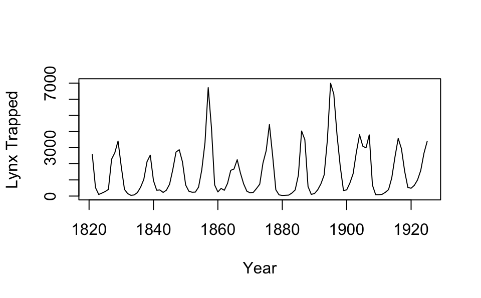
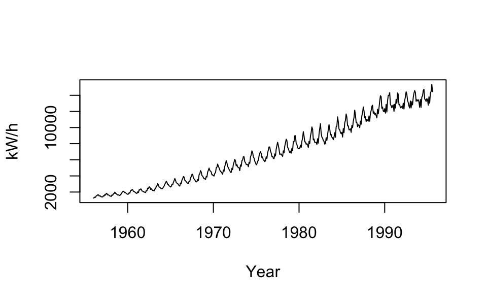
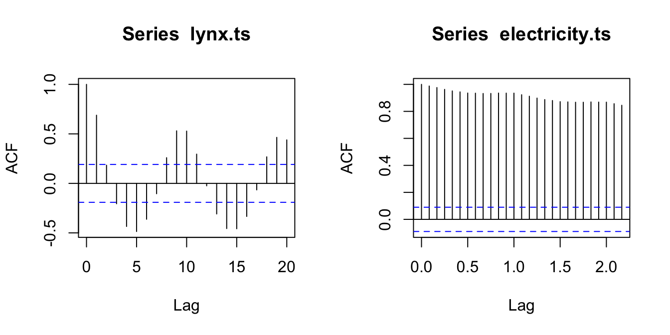
Lynx trapped ACF plot (left) and kilowatts per hour in Australia ACF plot (right).
6.2.2 Parameters in ARIMA methods
Therefore, in an ARIMA model we will use three parameters: (p, d, q).
p: refers to the use of past values of the series. It specifies the number of lags used in the model. For example, AR(2) or, ARIMA(2,0,0) specifies the use of two lags of the series.
d: degree of differentiation. Differencing your current and previous values d times.
q: model error as a combination of q previous error terms.
ARIMA works best for long and stable series.
6.2.3 Non-seasonal ARIMA models
If we combine differencing and autoregression we obtain a non-seasonal ARIMA model: \[
y'_t = c + \phi_1y'_{t-1}+\cdots+\phi_py'_{t-p}+\theta_1\epsilon_{t-1}+\cdots+\theta_q\epsilon_{t-q}+\epsilon_t
\] where \(y'_t\) is the series to which differencing has been applied. These models are represented as ARIMA(\(p,d,q\)), where \(d\) represents the degree of differencing.
6.2.4 Auto-ARIMA model
In R we have functions that automatically calculate the parameter values of an ARIMA model.
The auto.arima() function is a modification of the Hyndman-Khandakar algorithm.
R’s auto.arima() function combines tests, and minimisations to obtain an ARIMA model. By default, it can use initial approximations to speed up the model search (approximation=TRUE/FALSE).
If this does not allow to find a good model (minimum AICc) a larger set of models can be searched with the argument stepwise=FALSE. See [@forecasting] for more on this topic.
To choose a custom model for a non-seasonal series, we will use the Arima() function as follows:
Draw the dataset and identify outliers.
Transform the data to stabilise the variance.
If the data is not stationary use differencing until it is.
Analyse ACF/PACF for an ARIMA(\(p,d,0\)) or ARIMA(\(0,d,q\)) model.
Try to pick your model and use AICc to find the best one.
Check that the residuals behave like white noise:
if this is not satisfied look for another model
if this is true, we can use the model to predict
6.3 A use case
If your time series is not stationary, you should take steps to make it stationary before applying time series analysis techniques like ARIMA, Holt-Winters, or other methods. Stationarity is a fundamental assumption for many time series models, and non-stationary data can lead to unreliable results. Here’s what you should do:
Identify Non-Stationarity:
First, ensure that you have identified the non-stationarity in your time series data. Common signs of non-stationarity include trends (long-term changes) and seasonality (repeating patterns).
or use Autocorrelation Function (ACF) and Partial Autocorrelation Function (PACF)
acf(time_series_data)pacf(time_series_data)
or use seasonal decomposition techniques (e.g., stl()) to break down your time series into its trend, seasonal, and residual components. If you observe strong trends or seasonality, it suggests non-stationarity.
The most common method to achieve stationarity is differencing. You can difference the data by subtracting each data point from the previous one (first-order differencing). Repeat this process until the data becomes stationary. For example, you can use the diff() function in R.
For instance:
# Example time series data (replace with your actual data)time_series_data <-c(100, 110, 105, 120, 130, 135, 140, 150)# First-order differencingfirst_order_difference <-diff(time_series_data, lag =1)# The 'first_order_difference' variable now contains the differenced values# Second-order differencingsecond_order_difference <-diff(time_series_data, lag =1, differences =2)# The 'second_order_difference' variable contains the result of second-order differencing# Print or visualize the differenced dataprint(first_order_difference)## [1] 10 -5 15 10 5 5 10print(second_order_difference)## [1] -15 20 -5 -5 0 5# Adjust the lag and differences parameters according to the specific characteristics of your data and the level of differencing needed to achieve stationarity.
Log Transformation:
In some cases, taking the logarithm of the data can help stabilize variance and reduce non-stationarity, especially when you have exponential growth.
For instance:
log_transformed_data <-log(original_data)
Seasonal Differencing:
If your data exhibits seasonality, consider seasonal differencing by subtracting values from the same season in the previous year or period.
For instance:
seasonal_difference <-diff(time_series_data, lag =12)
Remove Trends:
If you identify a trend in your data, remove it by fitting a trend model (e.g., linear or polynomial) and subtracting it from the data. You can also use rolling means or moving averages.
For instance:
library(tseries)first_order_difference <-diff(time_series_data, lag =1)
Use Seasonal Decomposition:
Seasonal decomposition techniques, like seasonal decomposition of time series (STL) or classical decomposition, can help in separating the trend and seasonality from the data.
Perform an Augmented Dickey-Fuller (ADF) test to quantitatively test for stationarity. The test determines whether your data is stationary or not. If the p-value is less than a chosen significance level (e.g., 0.05), you can consider the data stationary.
Select Appropriate Parameters:
Once the data is stationary, you can identify appropriate parameters (e.g., p, d, q) for ARIMA modeling.
Visual Inspection Systematically try different combinations of parameter values (p, d, q) and evaluate model fit. Expert Knowledge Use auto.arima()
Model Building and Forecasting:
With stationary data and appropriate parameters, you can proceed with building your time series model (e.g., ARIMA) and make forecasts.
Evaluate and Validate:
After modeling, evaluate your results, validate the model, and use it for forecasting or analysis.
Remember that the process of making a time series stationary may involve trial and error. It’s essential to understand the nature of your data and apply the appropriate transformations or differencing to achieve stationarity.
Additionally, some data may require more advanced techniques like seasonal adjustment, structural break analysis, or transformation of the underlying process to achieve stationarity.
6.4 Example
Analyse the evolution of the minimum temperatures since 2001 in Malaga with the methods seen in this document.
We obtain a time-series object with the ts function, as our data are divided into months, we set the parameter frequency to 12 and we indicate that we start in January 2001. Then we draw the object obtained:
library(readr)temperaturas <-read_csv( here::here("data","temp.csv"))## Rows: 214 Columns: 6## ── Column specification ────────────────────────────────────────────────────────## Delimiter: ","## chr (2): fecha, indicativo## dbl (4): X1, X1_1, tm_max, tm_min## ## ℹ Use `spec()` to retrieve the full column specification for this data.## ℹ Specify the column types or set `show_col_types = FALSE` to quiet this message.ts.p1 <-ts(temperaturas$tm_min, start =c(2001, 1), frequency =12)plot.ts(ts.p1, xlab ="años", ylab ="temperatura mínima", main ="Temperaturas mínimas Málaga")
ARIMA models
We decompose the data: Seasonal component, Trend component, Cycle component y residual.
we obtain a time series with a frequency of 12 months
descompose
decomposing the series and removing the seasonality can be done with seasadj() within the forecast package
obj.ts <-ts(na.omit(temperaturas$tm_min), frequency =12, start =c(2001, 1))decomp <-stl(obj.ts, s.window ="periodic") # uses additive model by defaultdeseasonal_cnt <-seasadj(decomp)plot(decomp)
Previously we have seen that the series is stationary, but to fit an ARIMA model requires the series to be stationary.
with ADF test we can know if it is stationary or not.
adf.test(obj.ts, alternative ="stationary")## Warning in adf.test(obj.ts, alternative = "stationary"): p-value smaller than## printed p-value## ## Augmented Dickey-Fuller Test## ## data: obj.ts## Dickey-Fuller = -14.33, Lag order = 5, p-value = 0.01## alternative hypothesis: stationary