4 Bayes

4.1 Bayesian probability theorems

If we recall the conditional probability:

\[\mathbb{P}(A|B) = \frac{\mathbb{P}(A\cap B)}{\mathbb{P}(B)}\] we will be able to write: \[\mathbb{P}(A\cap B) = \mathbb{P}(A|B)\cdot \mathbb{P}(B)\] and, since \(A\cap B = B\cap A\): \[\mathbb{P}(A\cap B) = \mathbb{P}(B|A)\cdot \mathbb{P}(A)\] This fact can be used to link \(\mathbb{P}(A|B)\) and \(\mathbb{P}(B|A)\): \[\mathbb{P}(A|B) = \frac{\mathbb{P}(B|A)\cdot \mathbb{P}(A)}{\mathbb{P}(B)}\] This result is known as Bayes’ theorem.

4.2 Bayesian Inference

When modelling a phenomenon, one uses parameters that describe the behaviour of the system.

For example, in the toss of a coin a given number \(n\) of times, knowing the number of times it comes up face depends directly on a parameter which is the probability \(p\) that the coin comes up heads in an isolated toss. In fact, the probability distribution of the number of heads in those \(n\) flips is a binomial \(B(n, p)\). Knowing \(p\), we can estimate the average number of heads in \(n\) flips.

Continuing with the example, after carrying out \(n\) tosses, obtaining \(k\) heads, we ask ourselves if the coin is balanced, that is, if \(p = 0.5\). In this case, we could approximate \(\hat{p} = \frac{k}{n}\), and we would use a hypothesis test on the proportion of successes (heads) in \(n\) trials: \[\begin{array}{rcl} H_0 &:& p = 0.5 \\ H_1 &:& p\ne 0.5\\ \end{array}\]

This is the so-called frequentist view of statistics.

Bayesian inference has a slightly different purpose, as the parameter is considered as another variable:

It is assumed that we have a priori knowledge about the distribution of the parameters of the phenomenon.
We have data that provide a credibility or likelihood of the parameter.
An a posteriori estimate of the probability distribution of the parameters is obtained, taking into account the data obtained.

All this is related by means of Bayes’ Theorem above. Let \(\theta\) be the parameter that models the phenomenon (for example, the probability \(p\) of getting heads when tossing a coin), and let \(D\) be the set of data obtained in an experiment of the phenomenon under study. Then: \[\mathbb{P}(\theta|D) = \frac{\mathbb{P}(D|\theta)\cdot \mathbb{P}(\theta)}{\mathbb{P}(D)}\] In short, it is usually written (since the denominator does not depend on \(\theta\)): \[\mathbb{P}(\theta|D) \propto \mathbb{P}(D|\theta) \cdot \mathbb{P}(\theta)\]

\(\mathbb{P}(\theta|D)\) is the posterior distribution of the parameter (once we have taken the experimental data into account), \(\mathbb{P}(D|theta)\) is the likelihood or credibility (what is the probability of having obtained the data we have obtained, knowing that the parameter has the value \(\theta\)), and \(\mathbb{P}(\theta)\) summarises the a priori knowledge about the parameter.

Bayesian inference can therefore be summarised as: \[\text{Posterior} = \text{Likelihood} \cdot \text{Prior}\]

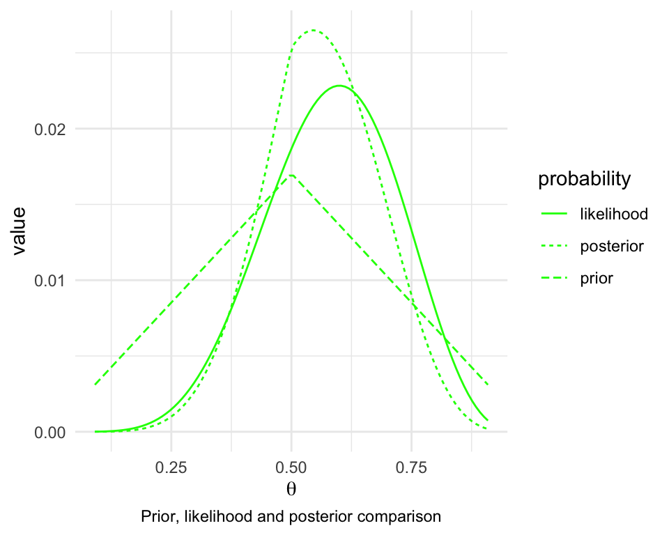
Given that the Prior can be prior knowledge or belief about the parameter distribution, then Posterior is the update of that knowledge or belief, taking into account the available evidence (which is represented by the term Likelihood).

4.3 Bayesian inference in `R`.

We show an example to demonstrate the connections between the three distributions described above. We are going to study the flips of a coin and what is the posterior probability of getting heads.

trials <- c('head', 'head', 'head', 'tail', 
             'tail', 'head', 'head', 'tail',
             'tail', 'head')
N <- length(trials)                      
nHeads <- sum(trials == 'head')  
nTails <- sum(trials == 'tail')

We do not know the value of \(\theta\), the probability of drawing heads, so we will consider 100 candidate values between 0 and 1:

theta <- seq(from = 1 / (N + 1), 
             to = N / (N + 1), 
             length = 100)

4.3.1 Choice of Prior

Sometimes the choice of prior depends on some belief or prior knowledge about the parameter. It can be completely devoid of information (e.g., assume that any value of the parameter is equally likely), or provide quite a lot of information (consider that the value of the parameter, for example, is around 0.5).

Let’s start by considering a prior with information: Let’s assume that \(\theta\) follows a triangular distribution, which takes the maximum (the mode) at \(\theta = 0.5\):

# Triangular
pTheta <- pmin(theta, 1 - theta)
# We normalise so that the sum is 1
pTheta <- pTheta / sum(pTheta)
# We could represent it graphically in a simple way with:
# plot(theta, pTheta)
# lines(theta, pTheta)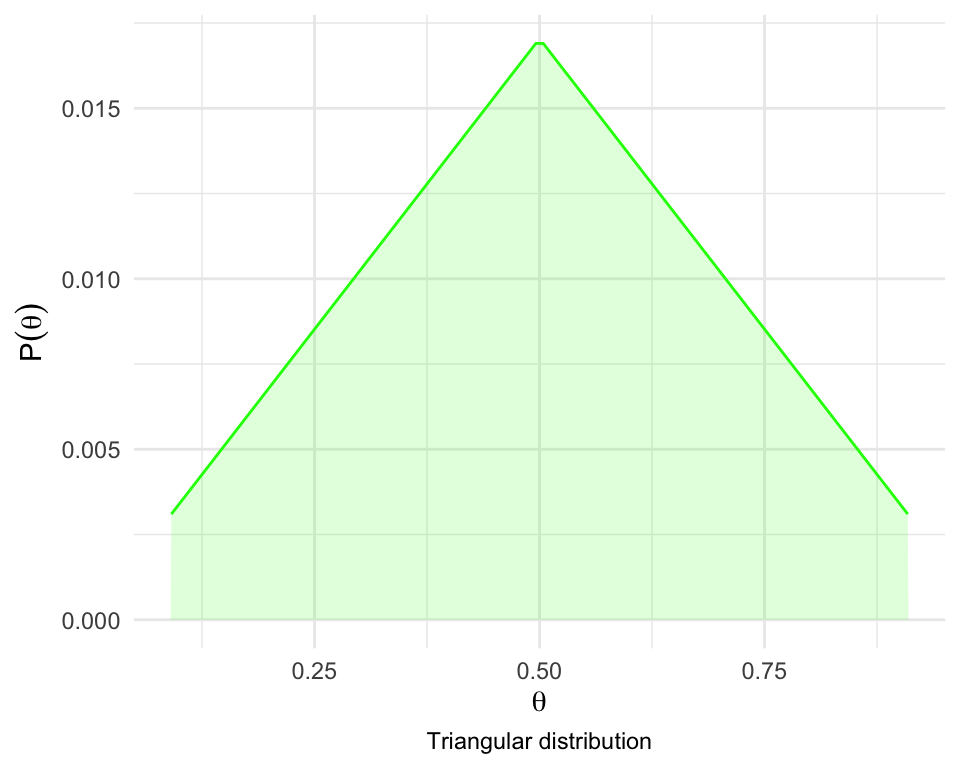

4.3.2 Likelihood function

In the frequentist view of statistics, our maximum likelihood estimate of the parameter \(\theta\) is the proportion of witnessed events over the total number of samples: \[\hat{\theta} = \frac{\text{nHeads}}{N}\]

theta_hat <- nHeads / N
theta_hat
## [1] 0.6

In Bayesian inference, the likelihood function is used to redistribute the credibility of the a priori distribution according to the new evidence (the data).

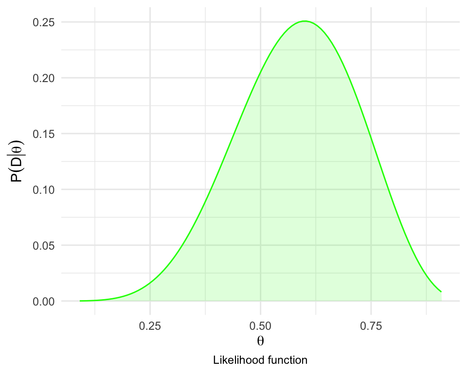
In this example, the likelihood function is given by a binomial distribution, which models how many successes occur among \(n\) attempts:

\[\mathbb{P}(\text{Roll }k\text{ heads out of }N\text{ trials}|\theta) = {N \choose k} \theta^k (1 - \theta)^{N - k}\]

\(N\): number of times the event could occur, i.e. the number of attempts.
\(k\): number of times the event occurs.
\(\theta\): the parameter of our model, which indicates the probability that in an isolated roll it comes up heads (Bernoulli experiment).

pDataGivenTheta <- choose(N, nHeads) * theta^nHeads * (1 - theta)^nTails

The likelihood has this approximate form:

4.3.3 Computation of the posterior distribution

The posterior distribution is computed from the prior using Bayes.

Recall that the denominator term in Bayes’ theorem is \(\mathbb{P}(D)\), the marginal probability of the data. By the total probability theorem, we can compute it this way: \[\mathbb{P}(D) = \int_0^1\mathbb{P}(D | \theta)\cdot\mathbb{P}(\theta)\mbox{d}\theta\] Having discretised the possible values of \(\theta\), this integral is left as a sum: \[\mathbb{P}(D) \approx \sum_i\mathbb{P}(D | \theta_i)\cdot\mathbb{P}(\theta_i)\]

# Marginal probability of data
pData <- sum(pDataGivenTheta * pTheta)  
# Bayes Theorem
pThetaGivenData <- pDataGivenTheta * pTheta / pData

Graphically:

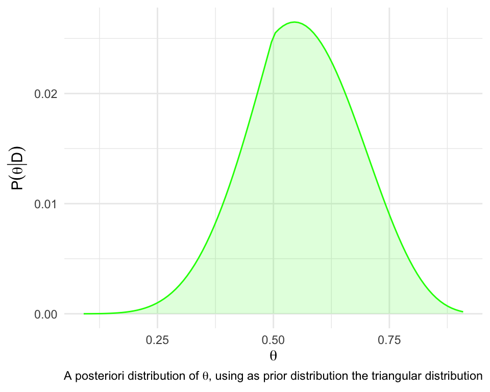
If we scale the likelihood function, we can see how the probability of the prior has been spread to resemble the new evidence (the likelihood or likelihood) and construct the a posteriori probability distribution of the \(\theta\) parameter:

By setting it as a table, we can inspect those rows close to the one we are interested in, which is the one where the posterior is maximum:

df1 <- data.frame(theta = theta,
                  prior = pTheta,
                  likelihood = pDataGivenTheta,
                  posterior = pThetaGivenData)

# id stores the row with the maximum "posterior".
id <- which.max(df1$posterior)
kable(df1[(id - 3):(id + 3), ], row.names = FALSE)

theta	prior	likelihood	posterior
0.5206612	0.0163380	0.2208619	0.0261323
0.5289256	0.0160563	0.2264357	0.0263299
0.5371901	0.0157746	0.2315250	0.0264494
0.5454545	0.0154930	0.2360913	0.0264894
0.5537190	0.0152113	0.2400985	0.0264492
0.5619835	0.0149296	0.2435132	0.0263286
0.5702479	0.0146479	0.2463052	0.0261280

The maximum a posteriori estimator is a point estimator of \(\theta\). We could use the mode or mean, for example, of this distribution just calculated, to give an estimate of the parameter value:

# Using mode:
theta_estimated_mode <- theta[which.max(pThetaGivenData)]
theta_estimated_mode
## [1] 0.5454545

# Using the mean or expectation:
theta_estimated_mean <- sum(theta * pThetaGivenData)
theta_estimated_mean
## [1] 0.5619734

4.3.4 Influence of the Prior.

Let’s start by using a prior that does not provide much information. We are talking about the fact that we do not know what the a priori value of \(\theta\) might be and what we do is to assign the same probability to all possible values, using the uniform distribution:

# Uniform: No information
pTheta <- dunif(theta)
# We normalise so that the sum is 1
pTheta <- pTheta / sum(pTheta)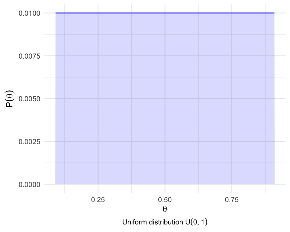

We repeat the above steps, resulting in the following a posteriori distribution:

# Marginal probability of data
pData <- sum(pDataGivenTheta * pTheta)
# Bayes Theorem
pThetaGivenData <- pDataGivenTheta * pTheta / pData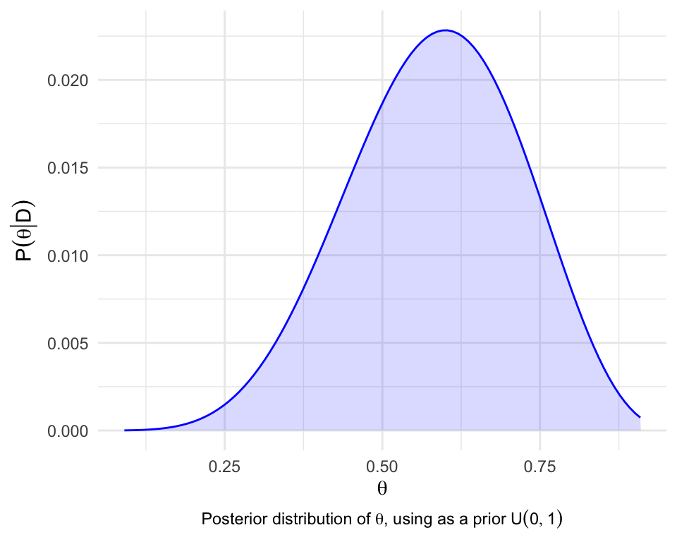

# Using mode:
theta_estimated_mode <- theta[which.max(pThetaGivenData)]
theta_estimated_mode
## [1] 0.6033058

# Using the mean or expectation:
theta_estimated_mean <- sum(theta * pThetaGivenData)
theta_estimated_mean
## [1] 0.5828379

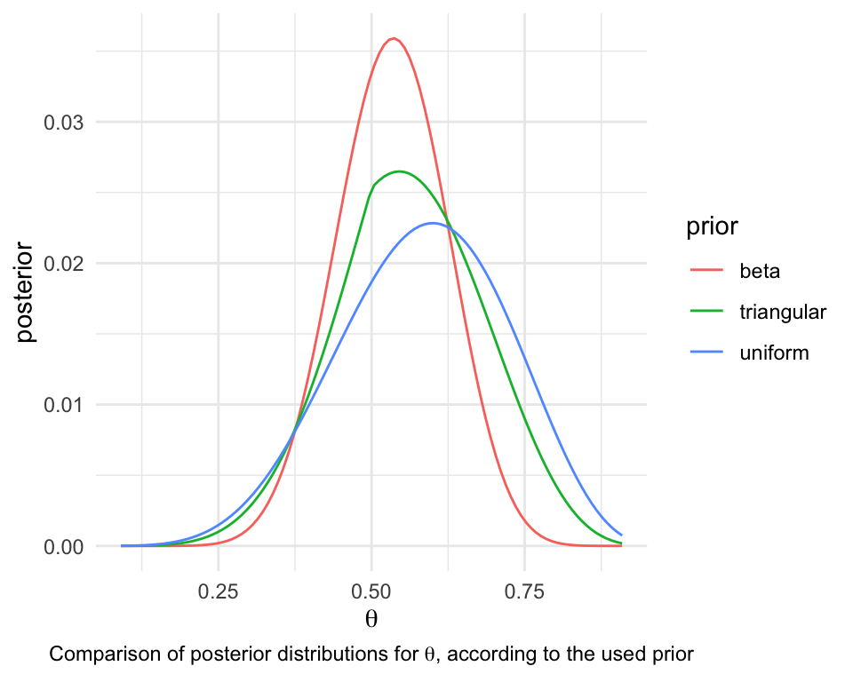
Notice that, when the prior is not informative, the posterior resembles the frequentist approximation \(\hat{\theta} = 0.6\).

Let us now use another a priori distribution, the beta of parameters 10, 10, which turns out to be very similar to a normal one, with mean 0.5:

# Beta distribution with mean 0.5
pTheta <- dbeta(theta, 10, 10)
# We normalise so that the sum is 1
pTheta <- pTheta / sum(pTheta)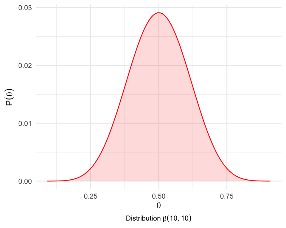

In this case

# Marginal probability of data
pData <- sum(pDataGivenTheta * pTheta)
# Bayes theorem
pThetaGivenData <- pDataGivenTheta * pTheta / pData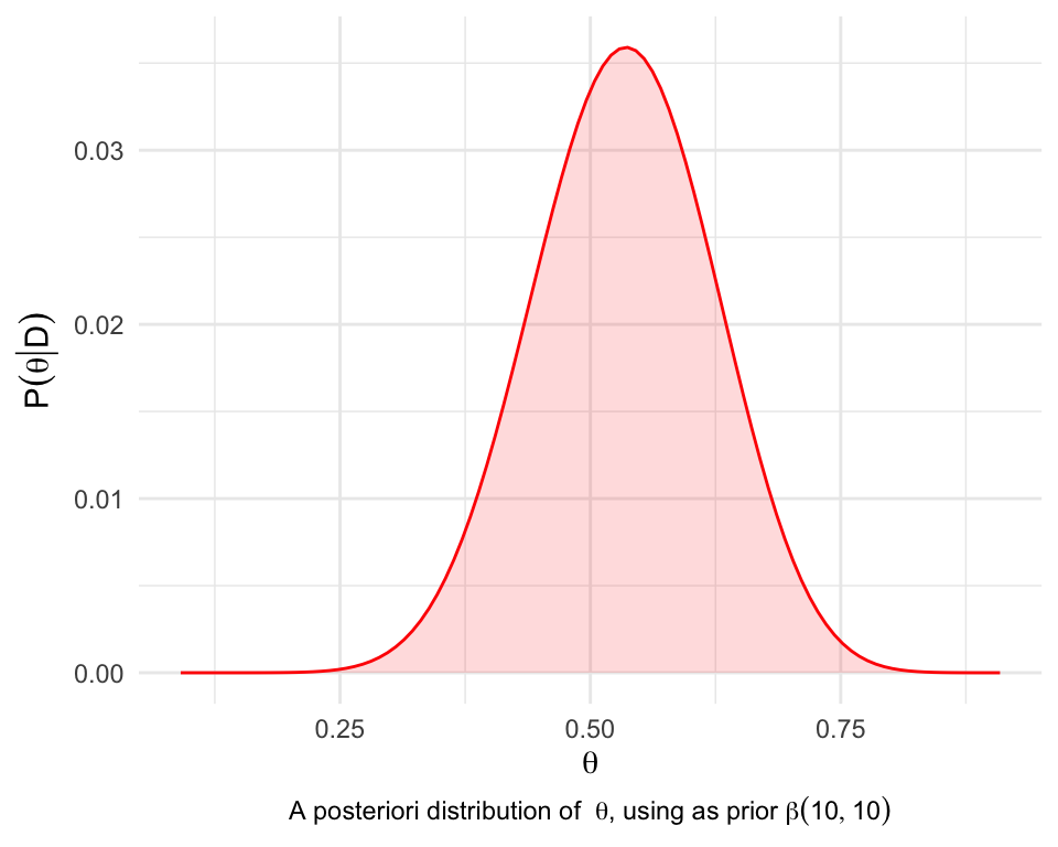

# Using mode:
theta_estimated_mode <- theta[which.max(pThetaGivenData)]
theta_estimated_mode
## [1] 0.5371901

# Using the mean:
theta_estimated_mean <- sum(theta * pThetaGivenData)
theta_estimated_mean
## [1] 0.5333333

We can see the a posteriori distributions according to the different prior in the following figure:

4.4 Interval estimation

A \(100(1 - \alpha)\) credibility interval is any interval \((a, b)\) such that \(\mathbb{P}(a < \theta < b | D) = 1 - \alpha\).

The shortest credibility interval is called the interval of maximum a posteriori density.

From R, we need the HDInterval package (installed with install.packages("HDInterval")), and it is used as follows:

library(HDInterval)
density <- data.frame(x = theta,
                      y = pThetaGivenData)
class(density) <- "density"

# By default, it considers 95% intervals
interval <- hdi(density, credMass = 0.95)
interval
##     lower     upper 
## 0.3553719 0.7024793 
## attr(,"credMass")
## [1] 0.95
## attr(,"height")
## [1] 0.005423003

This means that the interval of maximum a posteriori density (at 95%) is \((0.3553719, 0.7024793)\):

\[\mathbb{P}(0.3553719 < \theta < 0.7024793 | D) = 0.95\]

We can check this in R, since \[\mathbb{P}(a < \theta < b | D) = \int_a^b f(\theta | D)\mbox{d}\theta\] where \(f(\theta | D)\) is the a posteriori density function. In the discrete case: \[\mathbb{P}(a < \theta < b | D) \approx \sum_{a<\theta_i<b} \mathbb{P}(\theta_i | D)\] So:

lower_interval <- interval["lower"]
upper_interval <- interval["upper"]
# Probability of theta in that interval
# It should be approximately 0.95.
p <- sum(pThetaGivenData[(theta > lower_interval) & (theta < upper_interval)])
p
## [1] 0.9426559

4.5 Bayesian hypothesis testing

Suppose we have two hypotheses \(H_0\) (null) and \(H_1\) (alternative) that we want to compare. Before conducting any experiment, we may have beliefs about which of these hypotheses is true. After conducting an experiment, Bayesian inference talks about the probability that the null hypothesis is true (\(\mathbb{P}(H_0)\)), and even the a posteriori probability of the hypotheses, which can be calculated using Bayes’ Theorem: \[\mathbb{P}(H_0|D) = \frac{\mathbb{P}(D|H_0)\mathbb{P}(H_0)}{\mathbb{P}(D)}\] and the analogous for the alternative hypothesis \(H_1\).

Operating with the posterior distributions, we arrive at: \[\begin{array}{ccccc} \frac{\mathbb{P}(H_1|D)}{\mathbb{P}(H_0|D)} & = & \frac{\mathbb{P}(D|H_1)}{\mathbb{P}(D|H_0)} & \times & \frac{\mathbb{P}(H_1)}{\mathbb{P}(H_0)} \\ \uparrow & & \uparrow & & \uparrow \\ \text{posterior odds} & & \text{Bayes factor} & & \text{prior odds} \\ \end{array}\]

The prior odds ratio tries to quantify what is believed a priori about the two hypotheses. If it is a high value, it indicates that there is a strong belief that the hypothesis is true. Analogously, the posterior odds ratio is interpreted on the a posteriori evidence.

The factor relating the two is the Bayes factor (\(BF\)), which plays a similar role to the \(p\)-value in frequentist hypothesis testing: it quantifies the strength of the evidence provided by the data.

Thus, in a Bayesian analysis, the Bayes factor is often referred to when testing. The reason why the BF is mentioned instead of the posterior odds ratio is that the latter is dependent on the prior chosen by each researcher or data analyst. To eliminate this bias, the BF is used.

Interpretation of the Bayes Factor

An intuitive explanation of the Bayes factor is as follows: if you run an experiment and, for example, \(BF = 4\), this means that the data support that the alternative hypothesis is 4 times more likely than the null hypothesis.

In the following table, we show some interpretation of the \(BF\) about the evidence it implies in favour of the alternative hypothesis.

Bayes Factor	Interpretation
\(0 < BF < 3\)	Negligible evidence
\(3 < BF < 20\)	Positive (weak to moderate) evidence
\(20 < BF < 150\)	Strong Evidence
\(BF > 150\)	Very Strong Evidence

From R, the BayesFactor library can be used to calculate the Bayes factor from the data. In this case, the tests it performs for proportions are of the type: \[\begin{array}{c} H_0 : \theta = \theta_0 \\ H_1 : \theta \ne \theta_0 \\ \end{array}\]

To test whether \(\theta = 0.5\), just do:

library(BayesFactor)
## Warning: package 'BayesFactor' was built under R version 4.3.1
## Loading required package: coda
## Warning: package 'coda' was built under R version 4.3.1
## Loading required package: Matrix
## Warning: package 'Matrix' was built under R version 4.3.1
## ************
## Welcome to BayesFactor 0.9.12-4.5. If you have questions, please contact Richard Morey (richarddmorey@gmail.com).
## 
## Type BFManual() to open the manual.
## ************

# First argument: number of successes in the N attempts
# Second argument: the total number of attempts
# p is the value of theta in the null hypothesis
proportionBF(nHeads, N, p = 0.5)
## Bayes factor analysis
## --------------
## [1] Alt., p0=0.5, r=0.5 : 0.6908793 ±0%
## 
## Against denominator:
##   Null, p = 0.5 
## ---
## Bayes factor type: BFproportion, logistic

The higher the BF (here it is less than 1), the greater the evidence against the null hypothesis. In this case, there is little or no evidence that the alternative hypothesis (\(\theta\ne 0.5\)) is true.